10.4 Weights Characteristics

In addition to creating and loading spatial weights, the Weights Manager also contains functionality to compute and visualize some important properties of the weights. This includes summary characteristics, as well as the visualization of the connectivity structure by means of a histogram, map, or graph.

10.4.1 Summary characteristics

Figures 10.11, 10.13, 10.14, and 10.15 show the summary properties for rook, queen, second order queen and inclusive second order queen weights computed for the Ceará example. These include both metadata as well as descriptive statistics computed from the weights.

The metadata include the type of weights, symmetry, the original spatial layer (file), the id variable, the order, and, for higher order contiguity, whether include lower orders is true or false.

The descriptive statistics consist of the number of observations, the min, max, mean, and median number of neighbors, as well as an overall measure of sparsity, in the form of the % non-zero.

For the four weights considered so far, there is an increasing degree of density, reflected in all the descriptive statistics. For example, the mean number of neighbors increases from 5.09 for rook, 5.43 for queen, 12.07 for second order queen, to 17.50 for inclusive second order queen.

10.4.2 Connectivity histogram

The Histogram button at the left-hand side of the bottom of the weights manager (Figure 10.9) produces a connectivity histogram. This shows the number of observations for each value of the cardinality of neighbors, i.e., how many observations have the given number of neighbors. The graph is illustrated in Figure 10.20 for the rook contiguity associated with the municipalities of Ceará. It is a standard GeoDa histogram, with a number of options available, most of which are generic (see Section 7.2.1), and some specific to the connectivity histogram.

The overall pattern is quite symmetric, with a mode of 5 (i.e., most municipalities have 5 rook neighbors), but quite a long tail to the right (i.e., a few municipalities have a much larger number of neighbors). In addition to the visual inspection, the usual statistics of the distribution can be added to the bottom of the table by means of the View > Display Statistics option. The descriptive statistics are the same as listed in the weights manager summary.

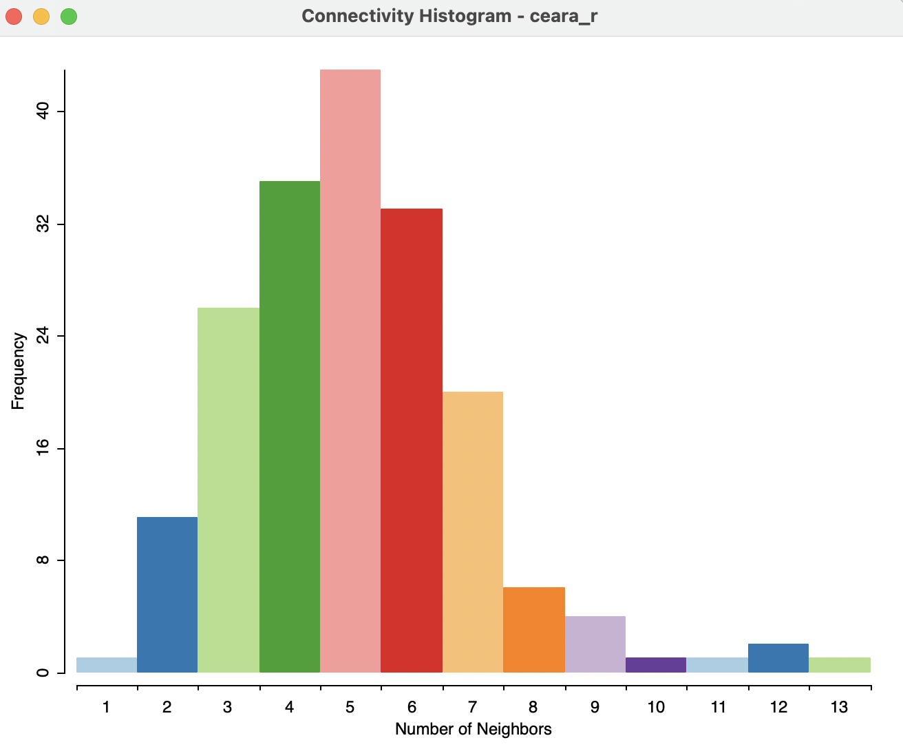
Figure 10.20: Rook contiguity histogram

Figure 10.21 illustrates the minor differences between rook and queen contiguity. In the histogram on the right, for queen contiguity, the municipalities with six neighbors are selected. In the linked contiguity histogram for rook weights on the left, the matching distribution is shown. Several of the observations with 6 neighbors using the queen criterion, have only 5 or even 4 neighbors for the rook criterion. This highlights the more inclusive nature of queen contiguity.

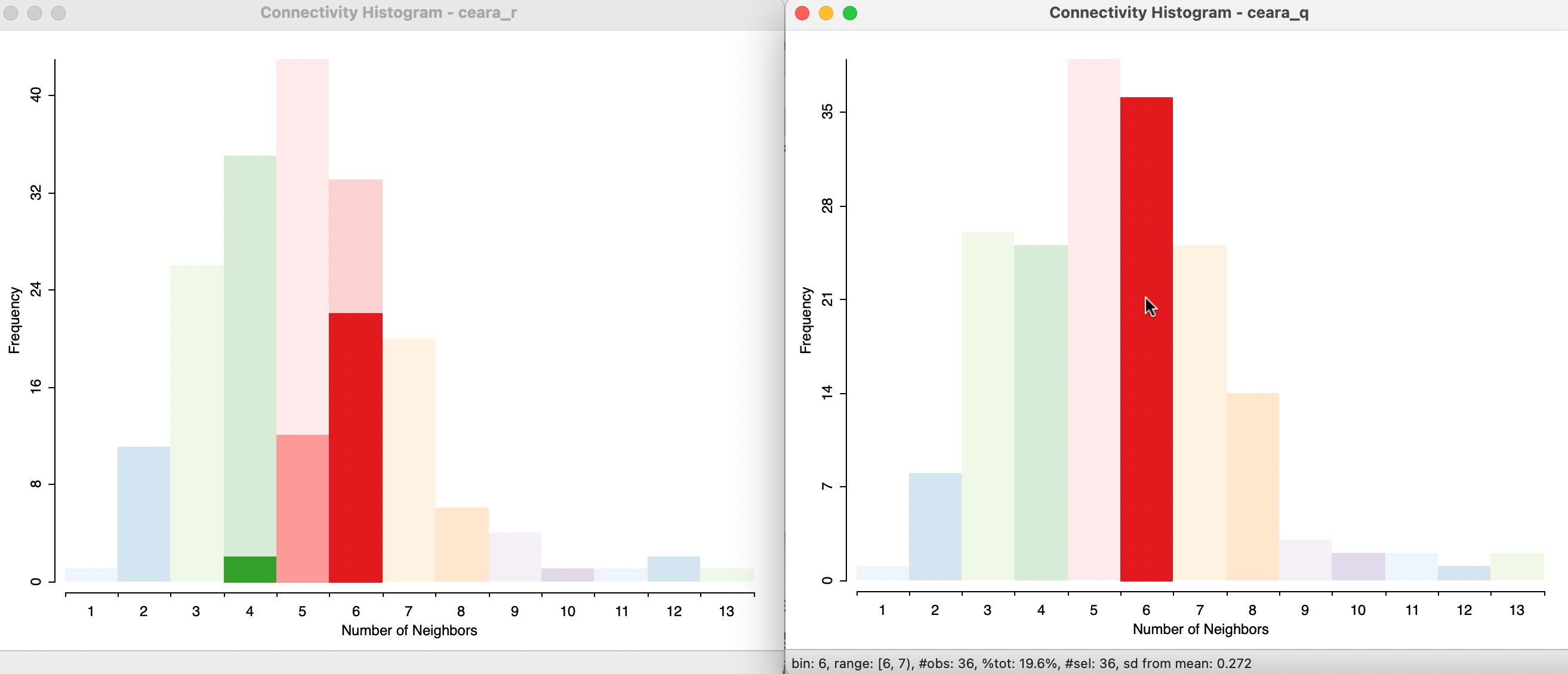
Figure 10.21: Rook and queen contiguity histograms

In addition, the contiguity histogram can be linked to any other window, such as the themeless map in the left-hand panel of Figure 10.22. In the contiguity histogram on the right (queen contiguity), the two observations with 13 neighbors are selected. A closer examination of the map identifies two very large areal units. Consequently, they will have more neighbors than the average sized unit.

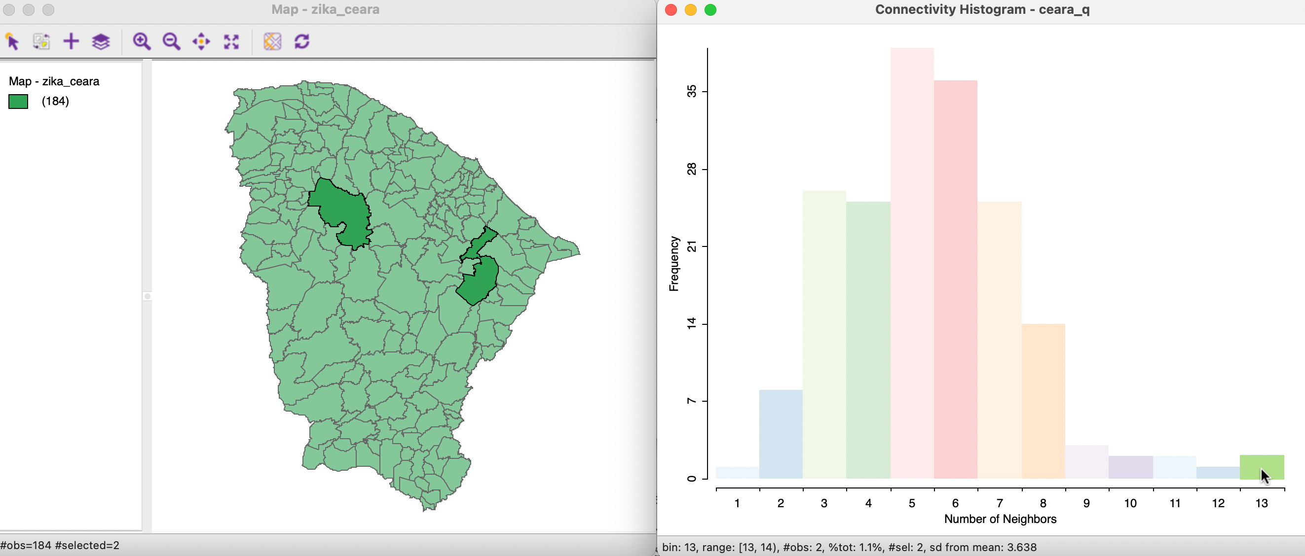
Figure 10.22: Linked contiguity histogram and map

It is good practice to check the connectivity histogram for any strange patterns, such as observations with only one neighbor, or neighborless observations (isolates, see Section 11.4.2).

Ideally, the distribution of the cardinalities should be smooth (i.e., no major gaps) and symmetric, with a limited range. Deviations from symmetry, such as bi-modal distributions (some observations have few neighbors and some have many) require further investigation. Any such characteristics will have an immediate effect on the corresponding weights, with implications for all the computations that use these weights.

10.4.2.1 Neighbor cardinality

A useful option of the connectivity histogram is to save the neighbor cardinality to the data table as an additional column/variable. This can then be used as an input in further analysis. For example, the number of neighbors is an important input into the calculation of the significance of the local join count statistic, covered in Chapter 19.

The Save Connectivity to Table option is invoked in the usual way by right clicking on the connectivity histogram window. This brings up a small dialog to specify the variable name (the default is NUM_NBRS).

10.4.3 Connectivity map

The middle button at the bottom of the Weights Manager interface (Figure 10.9) brings up a Connectivity Map. This is a standard GeoDa themeless map view, with all the usual features invoked through toolbar icons, including zooming and panning. In addition, the connectivity map includes a special functionality that highlights the neighbors of any selected observation. The window header lists the weights matrix to which the connectivity structure pertains.

In Figure 10.23, this is illustrated using queen contiguity for the Ceará municipalities. As soon as the pointer is moved over one of the observations, it is selected and its neighbors are highlighted. Note that this behavior is slightly different from the standard selection in a map, since it does not require a click to select. Instead, the pointer is in so-called hover mode. As soon as the pointer moves outside the main map, the complete layout is shown.

In the example, the selection is over the municipality of Santa Quitéria (code7 2312205), one of the two observations identified as having 13 neighbors. This outcome is listed in the status bar below the map, as well as the identifying codes for the neighbors. Moving the pointer to another observation immediately updates the selection and its neighbors.

The Connectivity Map in the weights manager is actually a special case of the Connectivity option in any map. This is considered in more detail in Section 10.4.5.1.

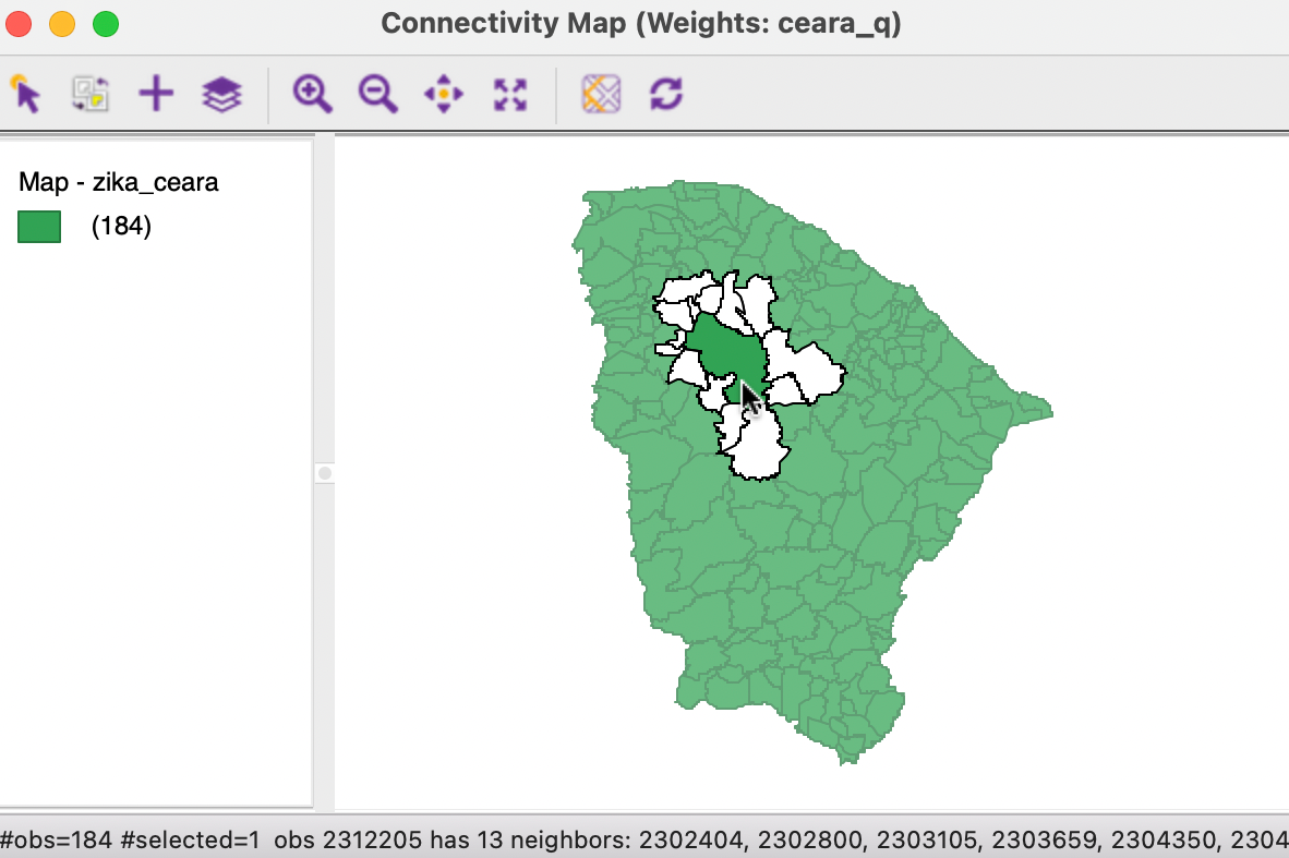
Figure 10.23: Connectivity map for queen contiguity

10.4.4 Connectivity graph

The right-most button at the bottom of the Weights Manager interface (Figure 10.9) brings up a Connectivity Graph. Like the connectivity map, this is a standard GeoDa map view, with all the usual options invoked through toolbar icons, including zooming and panning.

On additional feature is that the graph structure that corresponds to the spatial weights connectivity is superimposed on the map. For the queen contiguity in Ceará, this yields Figure 10.24. Again, the window header lists the corresponding spatial weights file (ceara_q).

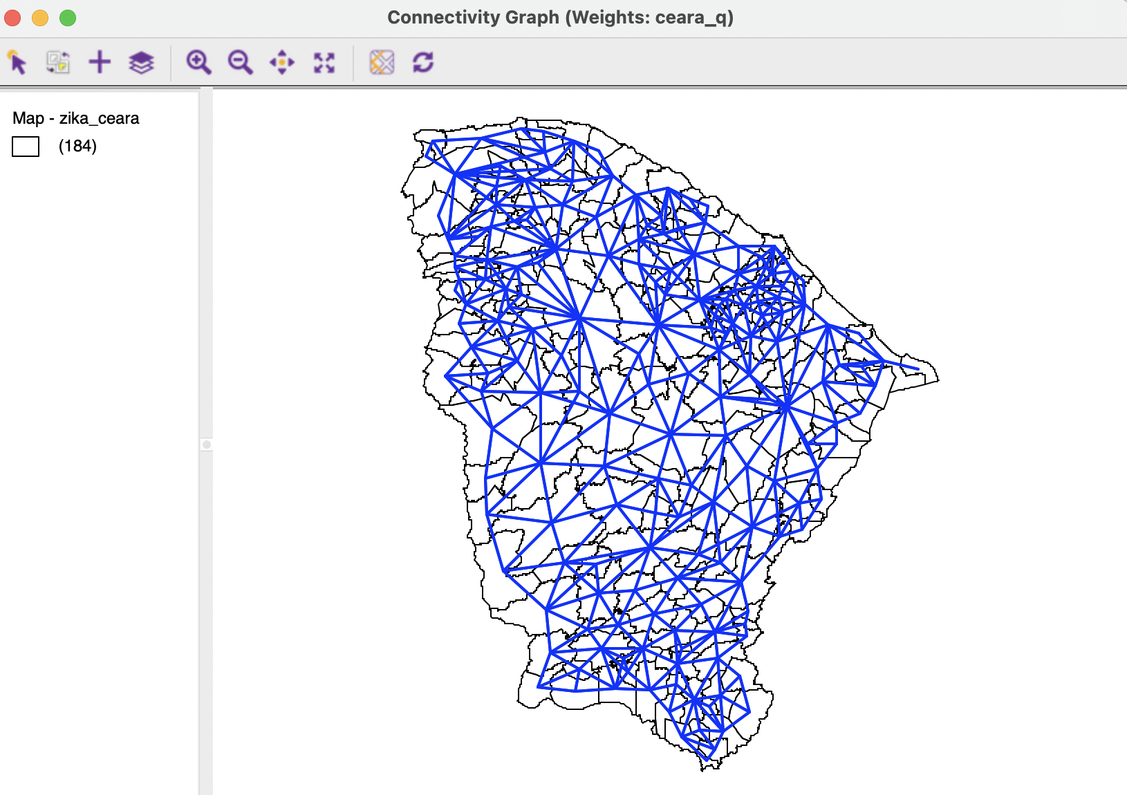
Figure 10.24: Connectivity graph for queen contiguity

As in the connectivity map, there are a few options that allow for some customization of the graph structure representation. These include the color and thickness of lines, and whether the background map is shown or not.

The default edge thickness is Normal, but two other options are available, to make the lines thicker (Strong) or thinner (Light). It is also often useful to change the color of the graph to something different from the default black. In Figure 10.24, these options have been used to change the thickness to Strong, the color to blue, the Opacity of the Fill Color to zero, and the Outline Color for Category to black.

The most dramatic of the options is the Hide Map feature. By checking this, the background map is removed and only the pure graph structure remains, as in Figure 10.25. This clearly brings out some interesting features of the graph, such as the observation with a single neighbor (a single edge in the graph) in the extreme north-east (highlighted in red).

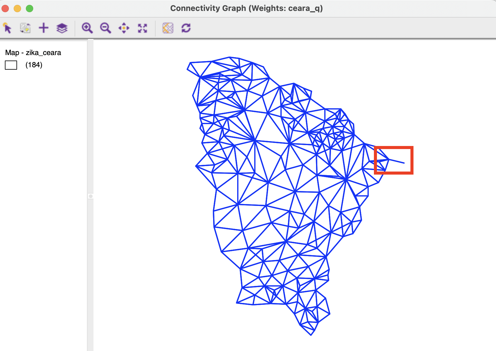
Figure 10.25: Connectivity graph for queen contiguity without map

10.4.5 Connectivity Option

Whenever there is an active weights matrix specified in the weights manager, the Connectivity Option becomes available in any map window as well as in the Selection Tool for the table.

10.4.5.1 Connectivity option in the map

In the discussion of the various map options in Section 4.5 of Chapter 4, the Connectivity option was deferred to the current chapter.

This option supports operations similar to those in a Connectivity Map, but applied to any current map. The functionality is invoked by selecting Connectivity > Show Selection and Neighbors from the options menu, in the usual fashion (right click).

With the option checked, the selection feature works the same as in the Connectivity Map. The main difference between the functionality in the Connectivity Map and the Connectivity option in any thematic map is that the latter is updated to the current active spatial weights file. In other words, as the active weights change, the connectivity structure is adjusted. In contrast, when selecting the Connectivity Map from the weights manager, there is only one such map, tied directly to the weights file from which it was invoked.

With the Show Selection and Neighbors option checked, it becomes possible to Change Outline Color of Neighbors, to Change Fill Color of Neighbors, and implement other cosmetic adjustments to the look of the selected polygons.

10.4.5.2 Connectivity option in the table

Neighbors of selected observations can also be displayed by means of a a feature of the table Selection Tool, as long as a weights matrix is active. The Add Neighbors to Selection button is central in the middle panel of of the Selection Tool in Figure 2.24 of Chapter 2.

This functionality requires that there is a current selection. Also, the Weights box must be specified. By default, the drop-down list will show the currently active weights, e.g., ceara_q.

Clicking on this button will add the neighbors of a current selection to the selection, similar to the operation of the Append to Current Selection option. Note that once the neighbors have been added, the current selection has grown to include those observations, so another Add Neighbors to Selection operation increases the selection set even more. This is not always what one has in mind.