9.2 Time Editor

The Time Editor is the mechanism through which different cross-sectional variables are grouped into a specific temporal sequence. In general, this could be any set of variables, but it is most relevant if the variables pertain to successive time periods. This requires that the observations for each time period are included in the data table as a separate cross-section. The design is that of a balanced panel, with the same cross-sectional units in each time period.⁶¹ The system is agnostic to the fact that the variables pertain to different time periods, so care must be taken to avoid counter intuitive situations (e.g., by selecting the wrong sequence of variables).

The space-time functionality is invoked from the menu as Time > Time Editor. The menu includes a separate item for each of the Time Editor and the Time Player. In contrast, when using the toolbar icon, i.e., the left icon in Figure 9.1, both are started.

The main purpose of the Time Editor dialog is to create grouped variables.

9.2.1 Creating grouped variables

The creation of grouped variables is a somewhat tedious process that involves identifying the variable names for each time period and combining them into a group. The interface, shown in Figure 9.2, consists of three major panels: Ungrouped Variables, New Group Details, and Grouped Variables. Each has a brief help window to explain the meaning of these terms, brought up by clicking on the ? symbol.

The left-most panel contains the variable names for all the numeric variables in the data table. They are selected by double clicking or by pressing on the arrow key (>). This moves the variable to the middle panel, where they are listed under Name. At the same time, the variables to include item is updated. The column associated with Time includes a period identifier, initially time 0, time 1, etc., but this can easily be edited. The name for the group is initially derived from the variable name entered, but also typically requires some further editing.

Individual variables can be moved up or down in the sequence (the sequence determines the order of the comparative statics graphs and maps) by selecting the variable and using the buttons at the bottom of the panel (Move Up and Move Down). In addition, any variable can be moved out of the grouping, back to the ungrouped variables list, by selecting it and clicking on the left arrow buttons (<).

When all the variables are included under New Group Details, in the correct order and with the correct Time label, another arrow key (to the right of the variable list) adds the group under the Grouped Variables list with the name as specified in the central panel. At this point, the process can be repeated for additional variables. However, for each grouped variable, the same number of original variables must be combined. In other words, the grouping always pertains to a fixed number of time periods, set when the first grouped variable is created.

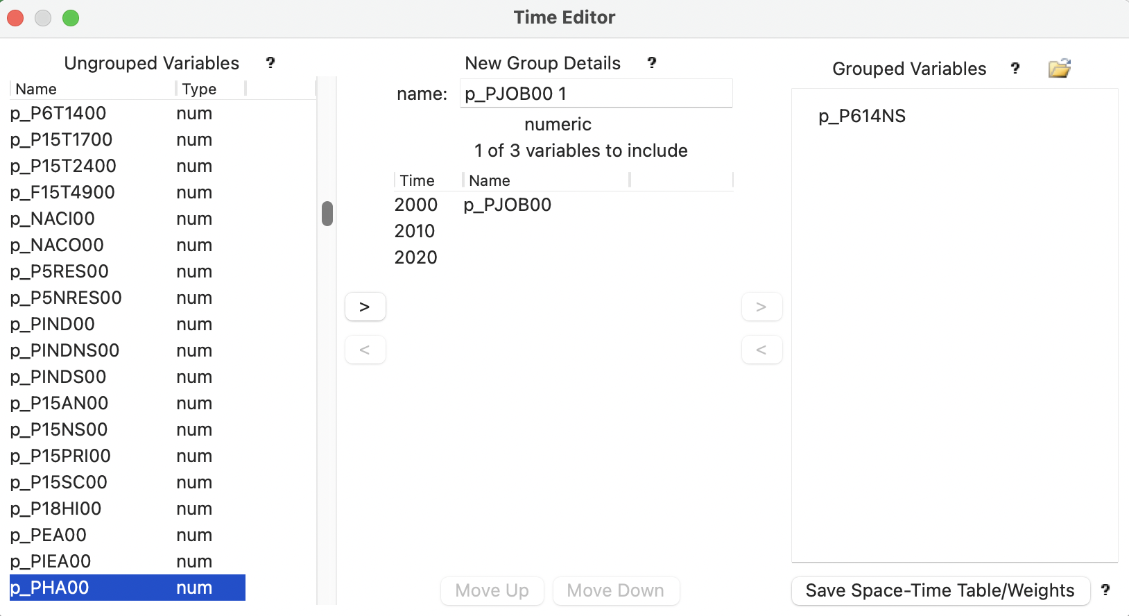
Figure 9.2: Time Editor interface

The example in Figure 9.2 is for the Oaxaca data set. It shows the situation after the variable p_P614NS (percentage of the population between 6 and 14 years of age that received no schooling) has been created by grouping p_P614NS00 (for 2000), p_P614NS10 (for 2010), and p_P614NS20 (for 2020). The Time labels have been set to 2000, 2010, and 2020. A new grouped variable is in the process of being created using p_PJOB00 for 2000 (percentage of the population over 12 years of age with a job). Note how the entry for name is not very useful at this point, and should be edited to p_PJOB, for example. The next variable to be selected should be p_PJOB10, for 2010.

To support a range of illustrations, two more groups are created: p_PHA (percentage of the population with access to health services), and p_CAR (percentage private inhabited dwellings with a car or van).

The grouped variables are shown in the data table with their new name, followed by the first time period in parenthesis. For example, in Figure 9.3, the entries are shown for p_PJOB and p_PHA.

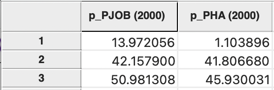
Figure 9.3: Grouped variables in data table

Note that the grouped variables have not been dropped as individual entries from the table, they are just not displayed as such. The new label in parentheses indicates that they have been grouped.

Finally, as mentioned, GeoDa is agnostic to what variables are grouped and in which order they are arranged, so this procedure can also be used to group variables that do not necessarily correspond to different time periods. For example, this may be useful when constructing a box plot graph that shows the box plots for multiple variables in one window.

9.2.1.1 Grouped variables in Project File

As discussed in the case of custom map categories (Section 4.6.3), any special definition such as a grouped variable will be lost if it is not saved in a project file (accomplished through File > Save Project). Once contained in a project file, the grouped variables can be re-used in later analyses. There can be several different project files associated with the same data layer, each focused on a special aspect of time dynamics.

The project file contains the time_ids specified in the time editor, and the new variable definitions under the group entry. For example, in Figure 9.4, the three years for the Oaxaca data set are included under the time_ids listing below the start of variable_order. Further down in the file, the group definitions for the p_PJOB and p_PHA variables are shown, together with some of the non-grouped variable definitions.

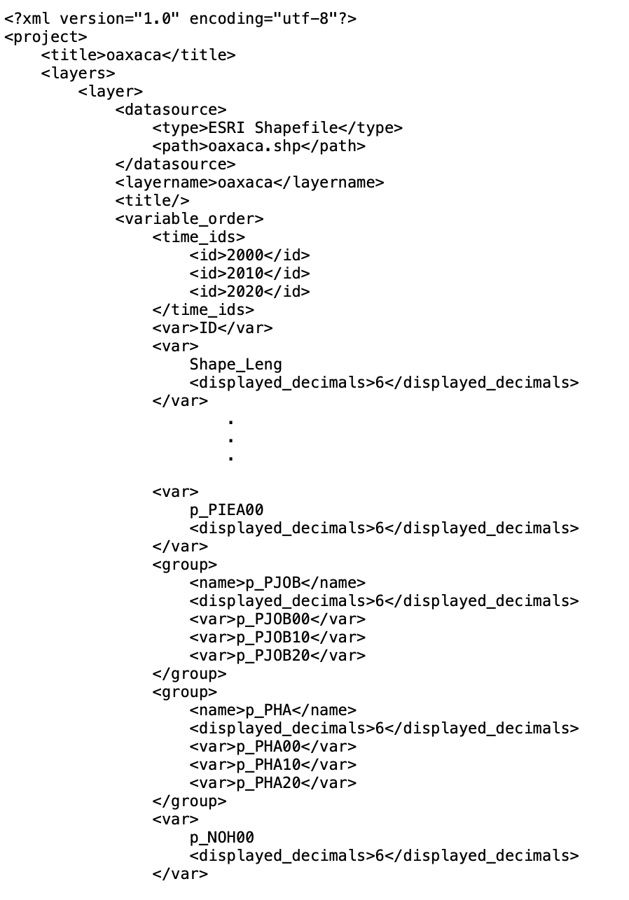
Figure 9.4: Grouped variables in project file

Note that the grouping of variables can only use one set of time periods, due to the synchronization mechanism that underlies the time player. So, in order to look at different time periods, such as two periods for one variable and three for another, two separate project files would need to be created. More precisely, any active grouping has to pertain to the same time labels for all the grouped variable. For example, in the Oaxaca data set, the poverty indicators pertain only to 2010 and 2020, whereas the census variables are for three years. In order to carry out any type of space-time analysis for the poverty indicators, a separate Time Editor operation would need to be carried out on a file that does not contain any other grouped variables (more precisely, one would need to start over). The new definitions should be saved in a different dedicated project file. Consequently, in the Oaxaca situation, there could need to be separate project files for a two-period analysis (2010 and 2020) and for a three period analysis (including 2000).

As seen before, instead of loading a spatial layer in the Connect to Data Source of the file open operation, one should load a project file with the gda extension. This will retain all grouped variable definitions contained in the project file.

9.2.1.2 Saving the space-time data table

A final option in the lower right hand side of the interface shown in Figure 9.2 is invoked by the Save Space-Time Table/Weights button. This creates a data file (typically in csv format) that contains a new space-time identifier, STID, as well as identifiers for the cross-sectional observation, the time period and time period dummy variables.⁶² The time grouped variables are stacked as cross-sections for each successive time period.

The space-time data file allows for pooled cross-section and time series analyses, but does not work with a corresponding map. In other words, the data can be loaded into a table for analysis (and, if appropriate, spatial weights included in the weights manager), but no map is available.

In addition, if a spatial weights file is active, a corresponding space-time weights GAL file is created as well, as detailed in Section 11.5.4.

---

61. An unbalanced panel would have different cross-sectional units by time period, which cannot be supported by GeoDa's current data structure.↩︎

62. When a spatial weights file is active, its ID variable is used as the cross-sectional identifier. In the absence of an active spatial weights file, a sequence of integer values is used.↩︎