17.4 Getis-Ord Statistics
An early class of statistics for local spatial autocorrelation was proposed by Getis and Ord (1992), and further elaborated upon in Ord and Getis (1995). It is derived from a point pattern analysis logic. In its earliest formulation, the statistic consisted of a ratio of the number of observations within a given range of a point to the total count of points. In a more general form, the statistic is applied to the values at neighboring locations (as defined by the spatial weights). There are two versions of the statistic. They differ in that one takes the value at the given location into account, and the other does not.
The \(G_i\) statistic consist of a ratio of the weighted average of the values in the neighboring locations, to the sum of all values, not including the value at the location (\(x_i\)). \[G_i = \frac{\sum_{j \neq i} w_{ij} x_j}{\sum_{j \neq i} x_j}\] In contrast, the \(G_i^*\) statistic includes the value \(x_i\) in both numerator and denominator: \[G_i^* = \frac{\sum_j w_{ij} x_j}{\sum_j x_j}.\] Note that in this case, the denominator is constant across all observations and simply consists of the total sum of all values in the data set. The statistic is the ratio of the average values in a window centered on an observation to the total sum of observations.
The interpretation of the Getis-Ord statistics is very straightforward: a value larger than the mean (or, a positive value for a standardized z-value) suggests a High-High cluster or hot spot, a value smaller than the mean (or, negative for a z-value) indicates a Low-Low cluster or cold spot. In contrast to the Local Moran and Local Geary statistics, the Getis-Ord approach does not consider negative spatial autocorrelation (spatial outliers).118
Inference can be derived from an analytical approximation, as given in Getis and Ord (1992) and Ord and Getis (1995). However, similar to what holds for the Local Moran and Local Geary, such approximation may not be reliable in practice. Instead, conditional random permutation can be employed, using an identical procedure as for the other statistics.
17.4.1 Implementation
The implementation of the Getis-Ord statistics is largely identical to that of the other local statistics. The Local G and Local G* options can be selected from the second group in the drop down menu generated by the Cluster Maps toolbar icon. Alternatively, they can be invoked from the menu as Space > Local G or Space > Local G*.
The next step brings up the Variable Settings dialog, followed by a choice of windows to be opened. The latter is again slightly different from the previous cases. The default is to use row-standardized weights and to generate only the Cluster Map. The Significance Map option needs to be invoked explicitly by checking the corresponding box. In contrast to previous cases, it is also possible to compute the Getis-Ord statistics using binary (not row-standardized) spatial weights, yielding a simple count of the neighboring values.
Continuing with the same example, using p_PHA10 (or p_PHA(2010)) from the Oaxaca data set, with queen contiguity weights, 99,999 permutations and p < 0.05 yields the significance and cluster maps for the \(G_i^*\) statistic shown in Figure 17.22. In this example, the results are identical to those for the \(G_i\) statistic, which is not shown separately.
Overall, 117 locations are identified as significant, the same total as for the Local Moran. In contrast to the latter, the cluster map for the Getis-Ord statistics only takes on two colors, red for hot spots (High-High), and blue for cold spots (Low-Low).
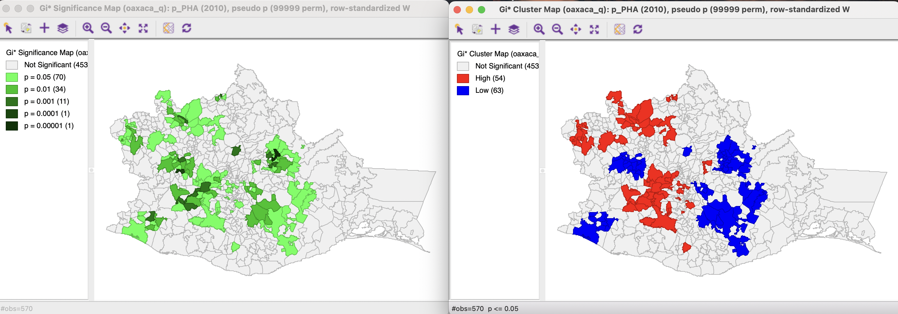
Figure 17.22: Gi* signficance map and cluster map
The options menu contains the same items as for the other local statistics, such as the randomization setting, the selection of significance levels, the selection of cores and neighbors, the conditional map option, as well as the standard operations of setting the selection shape and saving the image.
17.4.1.1 Saving the results
The Save Results option includes the possibility to save the statistic itself (G or G_STR), the cluster indication (C_ID) and the significance (PP_VAL). For the Getis-Ord statistics, there are only three cluster categories, with observations taking the value of 0 for not significant, 1 for a High-High cluster, and 2 for a Low-Low cluster.
17.4.2 Clusters and Outliers
The interpretation of High-High and Low-Low clusters for the Getis-Ord statistics is somewhat different from that of the Local Moran or Local Geary. As illustrated in Figures 17.23 and 17.24, the emphasis in the Getis-Ord statistics is on the magnitude of the neighbors.
The cluster maps on the right have, respectively, the observations in the High-High and Low-Low clusters selected. The corresponding observations are highlighted in the Moran scatter plot on the left.
In Figure 17.23, the High-High cluster observations all have spatial lags (average of neighbors) above the mean, whereas the variable itself takes values both above and below its mean. For the Low-Low cluster observations in Figure 17.24, all the spatial lags are below the mean, with again the variable itself taking values both above and below the mean.
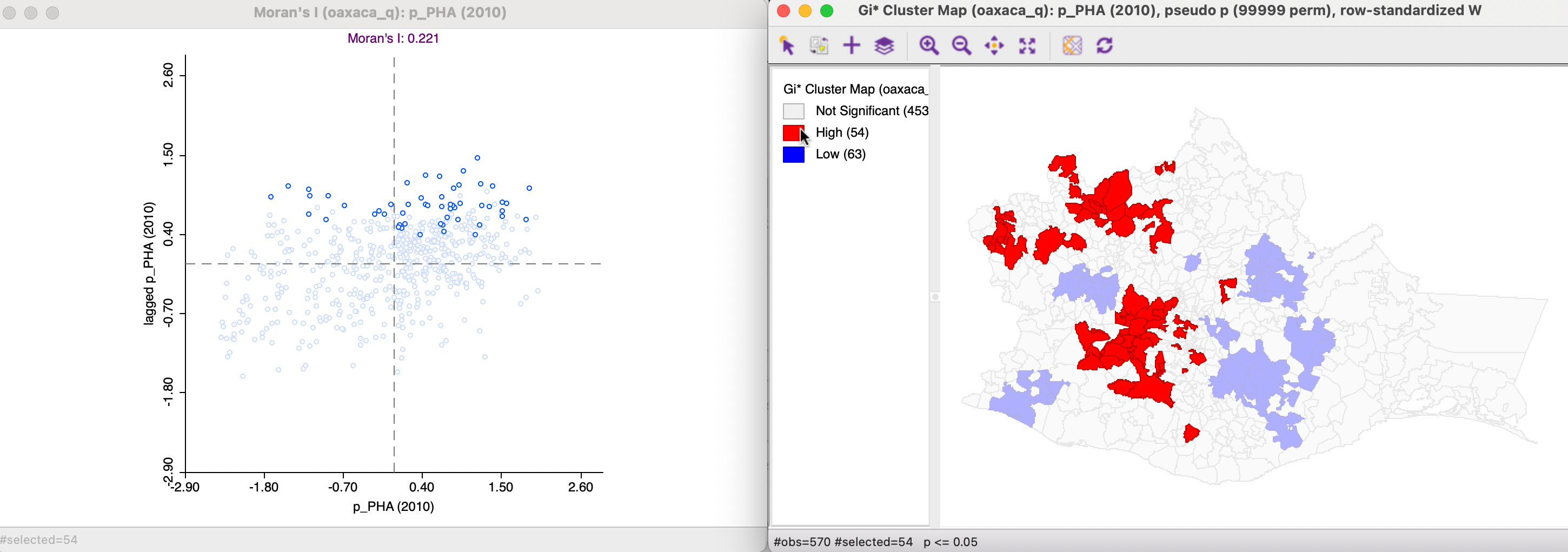
Figure 17.23: Gi* High-High clusters
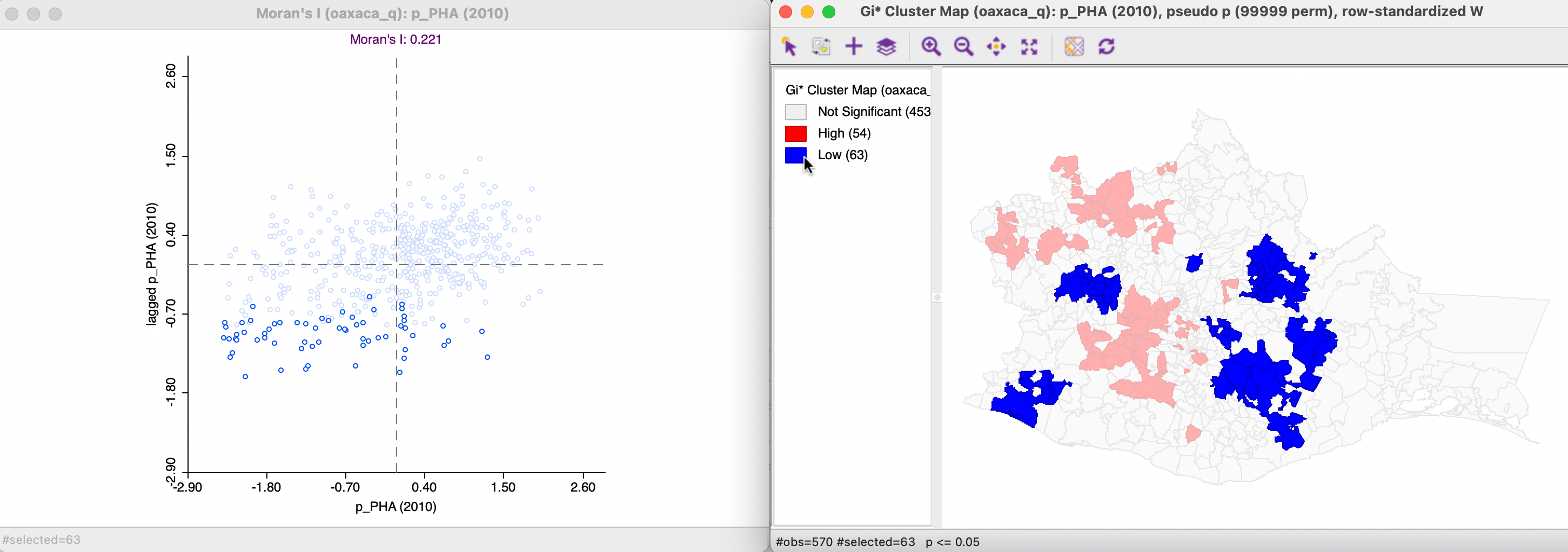
Figure 17.24: Gi* Low-Low clusters
Consequently, the Getis-Ord statistics include significant locations as High-High clusters that would be classified as Low-High spatial outliers according to the Local Moran. Similarly, the Getis-Ord statistics include significant locations as Low-Low clusters that would be classified as High-Low spatial outliers according to the Local Moran. The extent to which this affects the interpretation of the spatial extent of hot spots or cold spots depends on the relative importance of spatial outliers in the sample, but it can lead to quite different conclusions between the two types of statistics.
17.4.3 Comparing G Statistics and Local Moran
The Getis-Ord statistics typically identify the same locations as significant as the Local Moran, but their interpretation is different. This is primarily due to the fact that the Getis-Ord statistics do not account for spatial outliers. How much this affects results in practice depends on each particular instance, but it is something one should be aware of.
17.4.3.1 Clusters
Figures 17.25 and 17.26 show the hot spots and cold spots selected in the Getis-Ord cluster map on the right and identify the corresponding locations in the Local Moran cluster map on the left. As mentioned, all the significant locations match exactly, but their classification does not.
In Figure 17.25, the 54 hot spots in the Getis-Ord cluster map match the 42 High-High clusters in the Local Moran cluster map as well as the 12 Low-High spatial outliers, similar to what the Moran scatter plot in Figure 17.23 indicated.
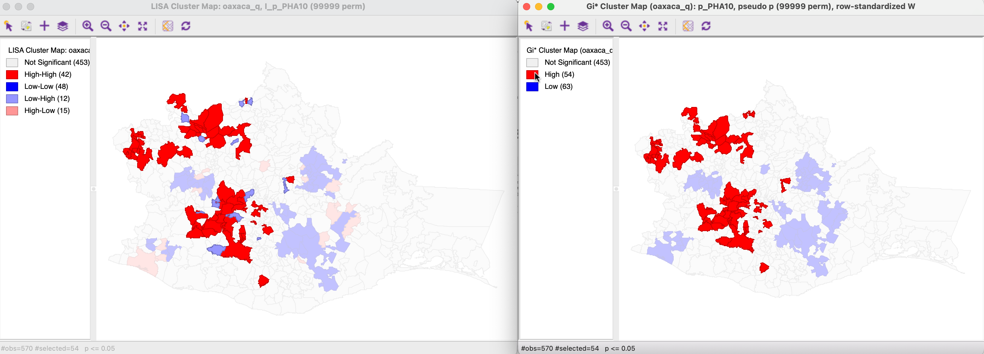
Figure 17.25: Gi* and Local Moran High-High clusters
On the other hand, in Figure 17.26, the 63 cold spots in the Getis-Ord cluster map correspond with the 48 Low-Low clusters in the Local Moran cluster map, in addition to the 15 High-Low spatial outliers. Again, this confirms the indication from the Moran scatter plot in Figure 17.24.
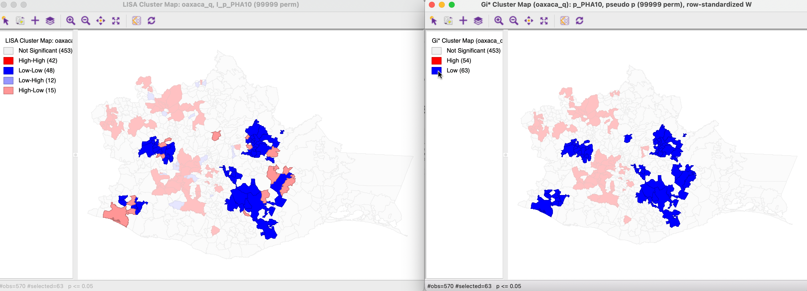
Figure 17.26: Gi* and Local Moran Low-Low clusters
17.4.3.2 Spatial outliers
Figures 17.27 and 17.28 illustrate the same properties, but approached from the significant spatial outliers in the Local Moran cluster map on the left.
In Figure 17.27, the 12 locations of significant Low-High spatial outliers are selected in the map on the left, and their corresponding observations identified in the Getis-Ord cluster map on the right. All locations are classified as High-High hot spots.
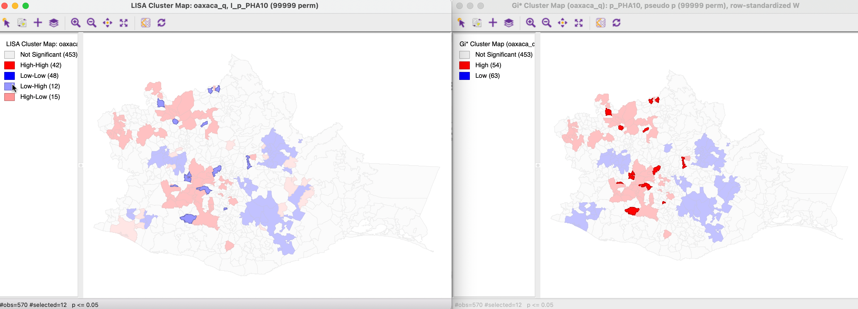
Figure 17.27: Gi* and Local Moran Low-High spatial outliers
In Figure 17.28, the reverse is illustrated. The 15 significant High-Low spatial outliers are selected in the Local Moran cluster map on the left. Their matching locations in the Getis-Ord cluster map on the right are all classified as Low-Low cold spots.
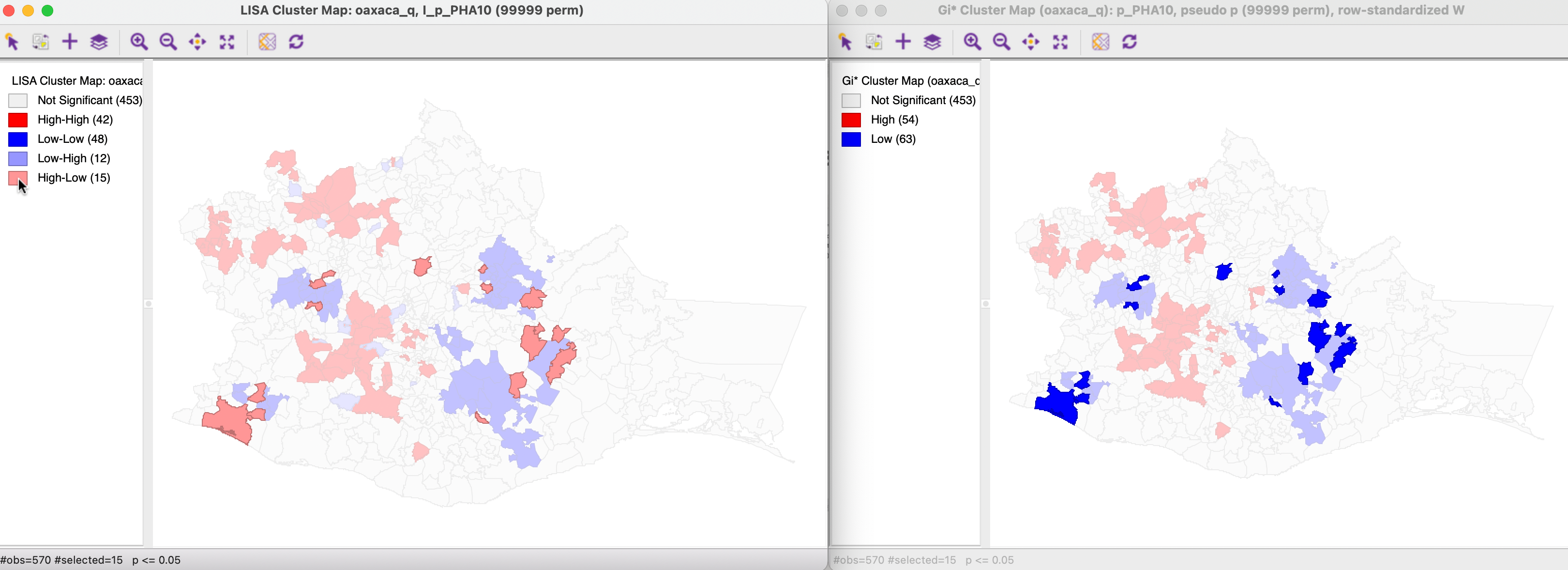
Figure 17.28: Gi* and Local Moran High-Low spatial outliers
When all observations for a variable are positive, as is the case in our examples, the G statistics are positive ratios less than one. Large ratios (more precisely, less small values since all ratios are small) correspond with High-High hot spots, small ratios with Low-Low cold spots.↩︎