5.3 Mapping Categorical Variables
In the discussion so far, the variable of interest (housing) was continuous, with a clear ordering from low to high. However, one often deals with indicator variables (0-1), or, even more generally, with variables that represent multiple categories. For the latter, each category is distinguished by a different integer value, but those values are typically not meaningful in and of themselves. Most importantly, the numerical values do not imply any ordering of the categories.
For a single variable under consideration, a map of its spatial distribution is created through the Unique Values Map option, the seventh item in the list in Figure 4.2. The functionality is illustrated with an indicator variable constructed from the cumulative incidence of Zika during the first three quarters of 2016 in the state of Ceará (zika_d).
A Co-location Map (eighth item in Figure 4.2) extends this to the comparison of multiple categorical variables, using the logic of map algebra (Tomlin 1990). This is illustrated with a comparison of the cumulative incidence of Zika (zika_d) with the presence of Microcephaly in the fourth quarter of 2016 (mic_d).
The Section closes with a brief discussion of issues associated with the extension to variables with more than two categories.
5.3.1 Unique values map
A map for a categorical variable is created by invoking Map > Unique Values Map and specifying the variable. Note that only variables that take on integer values are included in the drop down list.35
In the example in Figure 5.5, the categorical variable is zika_d. It only takes on the values of 1 (presence) and 0 (absence), reflected in the two colors in the map legend. The legend colors are generated from the ColorBrewer categorical map palette.36 As mentioned in Section 4.5.1, they can also be customized.
The map indicates that 32 of the 184 municipios had an incidence of Zika during the period under consideration. There seems to be a suggestion of a greater presence in the northern part of the state, with some groupings consisting of adjoining locations. A more formal assessment of these patterns is investigated in Chapter 19.
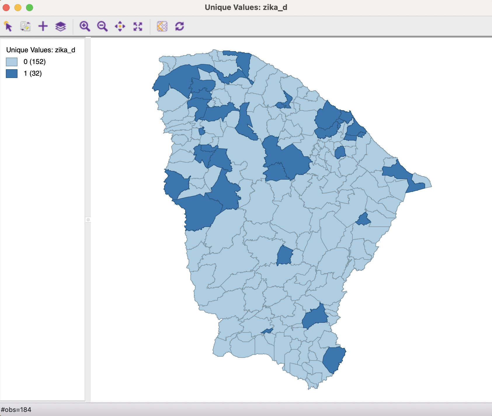
Figure 5.5: Unique values map, Zika indicator
All the standard map options apply to the unique values map. One additional option is to change the order (and color) of the categories. Since the categories are just that, and the numerical values associated with them do not imply any ordering, they can be changed. This is accomplished by grabbing the associated legend rectangle and moving it up or down in the list.
Such reordering can be handy in a so-called cluster map where the categories correspond to different cluster classifications. The comparison of two cluster maps can be facilitated by moving the categories around so that the same colors more or less correspond to the same locations.37
5.3.2 Co-location map
A co-location map combines the information from multiple categorical variables into a unique values map that shows those locations where the categories match. This is an example of map algebra, but applied to irregular spatial units rather than the more customary raster data.38
In essence, the process boils down to finding those locations where the codes for different categorical variables match. This is handled slightly differently for the simple case of binary variables and the more complex situation with multiple categories.
5.3.2.1 Binary categories
When the variables under consideration take on binary values, a co-location map can be constructed by hand as a unique values map of the product of the respective indicator variables. Only those locations that take on a value of 1 for all variables will be coded as one in the resulting unique values map.
However, a co-location map is different in that it also provides information on matches of locations with 0 for all variables, as well as on the locations of mismatches. In sum, rather than just two categories (match and no match), there are three: match of 1, match of 0, and mismatch.
The map is invoked in the usual way as Map > Co-location Map, which brings up a dialog to specify the different variables to be considered, as in Figure 5.6. The interface is used to select the variables, but also to choose the associated legend structure. Several options are provided, ranging from Unique Values, the suggested default in this case, to several customized legends associate with different types of maps (such as extreme values maps) and visualizations of spatial analyses (e.g., LISA Map, see Chapter 16).
In our example, the Unique Values default will do fine.
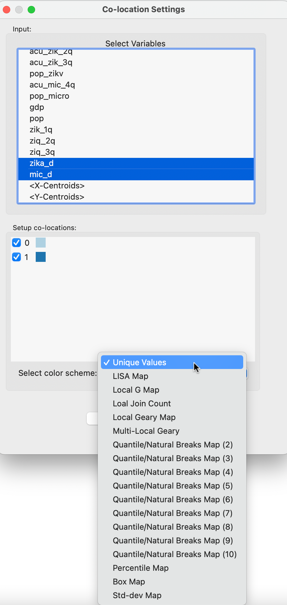
Figure 5.6: Co-location map variable selection, Zika and Microcephaly indicators
The two variables selected are indicator variables for the presence of respectively Zika (zika_d) and Microcephaly (mic_d). The corresponding co-location map is shown in Figure 5.7.
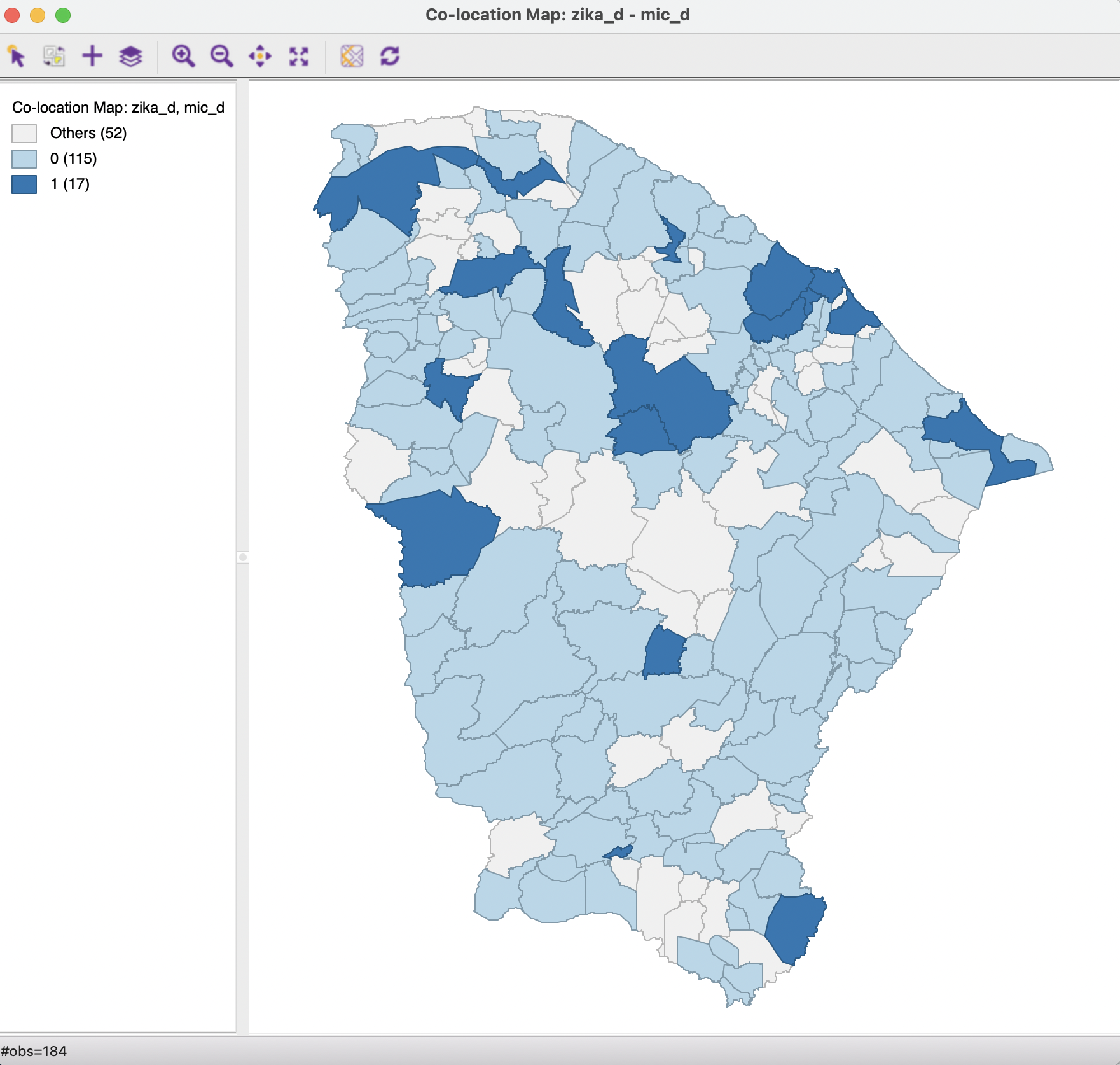
Figure 5.7: Co-location map, Zika and Microcephaly incidence
The legend contains three categories. One pertains to those locations with a common occurrence of 1 (17 observations), and another to those observations that share a value of 0 (115 observations). The third category (in grey) highlights the locations where there is a mismatch between the values (52 observations).
The logic of the co-location map is further illustrated in Figure 5.8. It shows the selected observations in each of the respective unique values maps that correspond to locations with a value of 1 in the co-location map. There are 17 observations selected in each of the maps. Clearly, these are the only locations where both maps have a dark blue color.
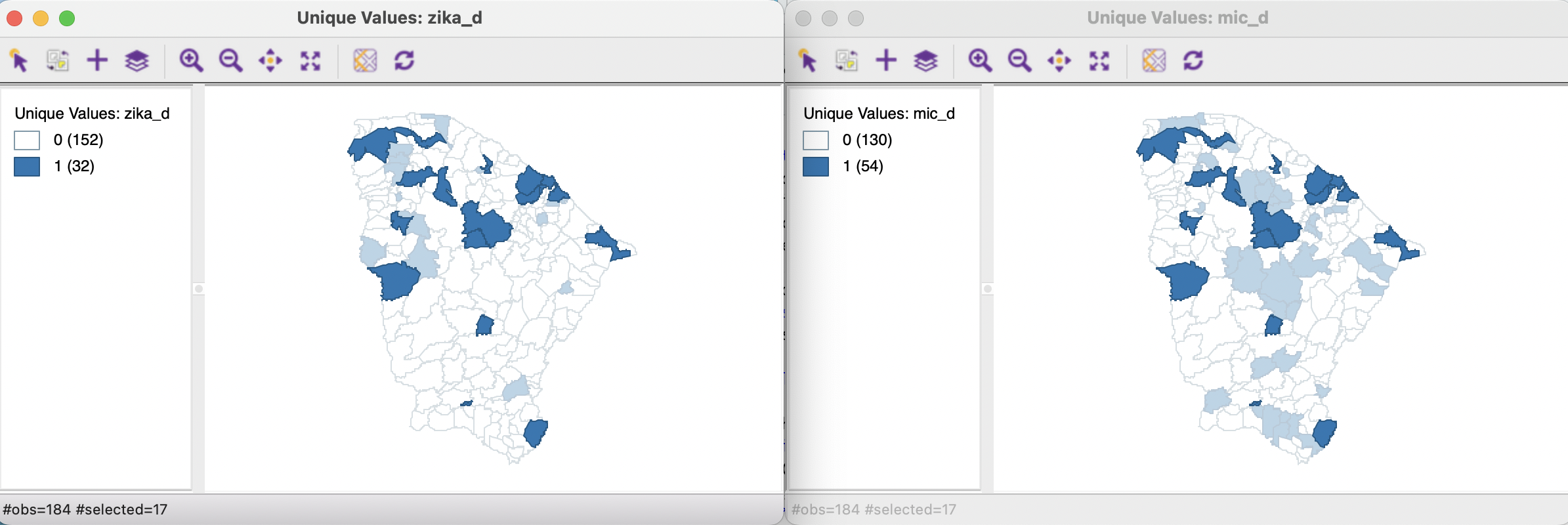
Figure 5.8: Selection of co-located observations
5.3.2.2 Multiple categories
When the variables pertain to multiple categories, the logic of the co-location map is the same, but it must be applied with caution. It is based on the equality of the categorical codes for each variable.
It is up to the user to ensure that the categories across variables are meaningful, since the co-location is based on the variables having the same code. For example, this is useful when comparing the extent to which the quartiles across different variables occur at the same locations. Or, to assess whether significant patterns of local spatial autocorrelation match across multiple variables. But it is also very easy to generate nonsensical results, for example, when the labels are not comparable.
One can change the label and color of a category by moving the legend rectangle up or down in the legend. This again highlights that the category values do not have any intrinsic numerical value.
If a variable that should be categorical appears to be missing from the list, it may have been formatted as real. This can be readily changed using Edit Variable Properties in the table, see Section 2.4.1.1.↩︎
http://colorbrewer2.org/#type=qualitative&scheme=Accent&n=3↩︎
This is covered in Volume 2.↩︎