12.3 Spatial Transformations
The main form of spatial transformation considered here is the so-called spatial lag operation. This summarizes the observations at neighboring locations into a single new variable. The weights matrix is central in this operation, since it identifies which observations need to be selected and if any weights need to be applied.
12.3.1 Spatially Lagged Variables
With a neighbor structure defined by the non-zero elements of the spatial weights matrix \(\mathbf{W}\), a spatially lagged variable is a weighted sum or a weighted average of the neighboring values for that variable (Anselin 1988). In the typical notation, the spatial lag of \(y\) is then expressed as \(Wy\).
Formally, for observation \(i\), the spatial lag of \(y_i\), referred to as \([Wy]_i\) (the variable \(Wy\) observed for location \(i\)) is: \[\begin{equation*} [Wy]_i = w_{i1}y_1 + w_{i2}y_2 + \dots + w_{in}y_n, \end{equation*}\] or, \[\begin{equation*} [Wy]_i = \sum_{j=1}^n w_{ij}y_j, \end{equation*}\] where the weights \(w_{ij}\) consist of the elements of the \(i\)-th row of the matrix \(\mathbf{W}\), matched up with the corresponding elements of the vector \(\mathbf{y}\).
In other words, the spatial lag is a weighted sum of the values observed at neighboring locations, since the non-neighbors are not included (those \(j\) for which \(w_{ij} =0\)). Typically, the weights matrix is very sparse, so that only a small number of neighbors contribute to the weighted sum. For row-standardized weights, with \(\sum_j w_{ij} = 1\), the spatially lagged variable becomes a weighted average of the values at neighboring observations.
In matrix notation, the spatial lag expression corresponds to the matrix product of the \(n \times n\) spatial weights matrix \(\mathbf{W}\) with the \(n \times 1\) vector of observations \(\mathbf{y}\), or \(\mathbf{W \times y}\). The matrix \(\mathbf{W}\) can therefore be considered to be the spatial lag operator on the vector \(\mathbf{y}\).
In a number of applied situations, it may be useful to include the observation at location \(i\) itself in the weights computation. This implies that the diagonal elements of the weights matrix must be non-zero, i.e., \(w_{ii} \neq 0\). Depending on the context, the diagonal elements may take on the value of one or equal a specific value, such as for kernel weights where the kernel function is applied to the diagonal.
An alternative concept of spatial lag is the so-called median spatial lag. Instead of computing a (weighted) average of the neighboring observations, the median is selected.
12.3.1.1 Creating a spatially lagged variable
The spatial lag computation is part of the Calculator functionality associated with a data table (Section 2.4.2). It is started from the menu as Table > Calculator, or by right clicking in a table to bring up the list of options.
The lag operation requires the Spatial Lag tab to be active. The Weight drop down list contains all the spatial weights available to the project, with the currently active weights listed. In the example illustrated in Figure 12.6, a time-enabled version of the Italian bank data is used, with the 6 k-nearest neighbor weights after intersection with the 73 km distance band. The spatial weights are contained in the file italy_banks_te_d73_k6.gal (see Section 11.6.1). The spatial lag operator will be applied to the variable SERV (2016), i.e., the time enabled ratio of net interest income over total operating revenues in 2016.
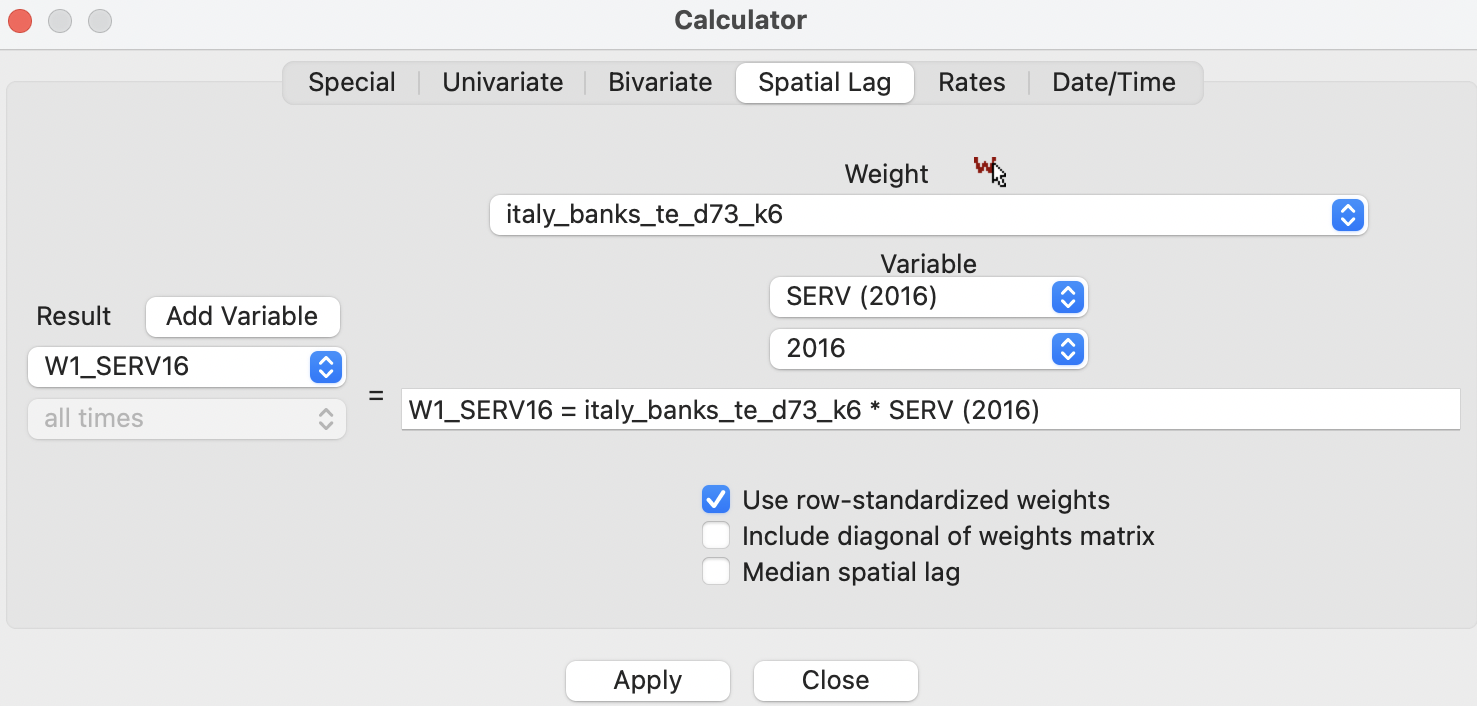
Figure 12.6: Spatial lag in calculator
To compute the spatially lagged variable, first Add Variable is selected to create a name for the new variable, W1_SERV16 in the example. At this point, the expression for the calculation of the lag is filled out in the box, listing both the weights and the original variable.
The default option is to Use row-standardized weights without including the diagonal elements. The result is added to the data table, as shown in Figure 12.6, in the column W1_SERV16.
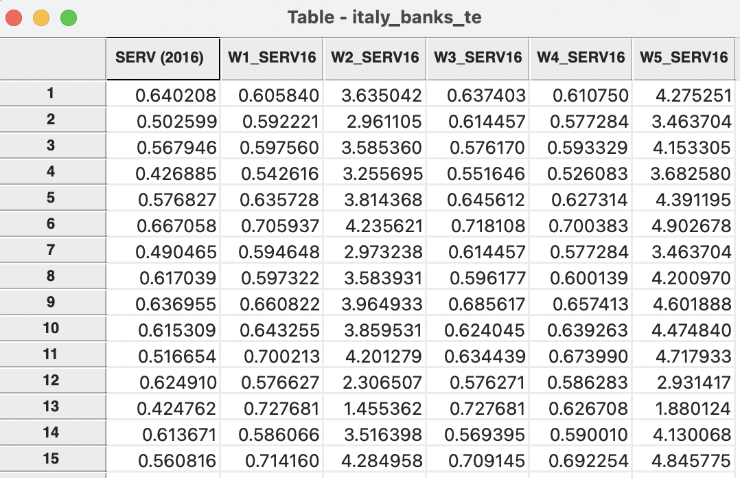
Figure 12.7: Spatially lagged variables added to table
The file italy_banks_te_d73_k6.gal contains the neighbor list for the first observation, with idd = 1. These are the observations with idd equal to, respectively, 64, 95, 96, 267, 272 and 309 (corresponding to table rows 15, 41, 42, 167, 172, and 209). The value of SERV (2016) for the first observation is listed as 0.640208. A look up in the data table reveals the values for the neighboring observations as 0.560816, 0.748250, 0.659608, 0.615197, 0.349620, and 0.701551. The average of these six values is 0.605840, which is exactly the entry on the first row of the W1_SERV16 column.
As illustrated in Section 11.6.1, the spatial weights intersection yields two isolates, observations with idd 269 (Valley of Aosta, row 169) and 287 (Sicily, row 187). Since a spatially lagged variable is undefined for an isolate (an actual computation would yield a value of zero), the corresponding entries in the table are empty. This avoids complications from mistakenly associating a value of zero in further calculations, such as in the computation of a spatial autocorrelation coefficient. The outcome of the empty entry is that the isolate observations are excluded from such computations.
The effect of the spatial lag operation is a form of smoothing of the original data. The mean is roughly the same (the theoretic expected values are the same), e.g., 0.6363 for the original variable vs. 0.6378 for the spatial lag, but the standard deviation is much smaller, i.e., 0.0943 for the original vs. 0.0562 for the spatial lag. Similarly, a form of shrinking has occurred: the original variable has a minimum of 0.3496 and a maximum of 0.9143, whereas for the spatial lag this has narrowed to 0.5124 to 0.7478.92
A measure of spatial correlation can be computed as the correlation between the original and the spatially lagged variable. Note that this is NOT the accepted notion of spatial autocorrelation considered in the literature (see Chapter 13). Nevertheless, as long as it is not interpreted in the context of a spatial autoregressive model, it remains a useful measure of the linear association between a variable and the average of its neighbors. In the example, this value is 0.350.93
12.3.1.2 Spatial lag as a sum of neighboring values
Combining different settings for the row-standardized and Include diagonal options allows for other notions of spatially lagged variables to be implemented. For example, a spatial lag as a sum of the neighboring values is obtained by unsetting all options.
The result is listed in column W2_SERV16 of the table (Figure 12.7). For the first observation, the corresponding value is 3.635042, which is the sum of the values for the six neighbors.
12.3.1.3 Median spatial lag
The Median spatial lag is obtained by checking the corresponding box (the two other options become unavailable). In the example, there are six neighbors, so the median is computed as the midpoint between the third (0.615197) and fourth (0.659608) values in the ranked set, yielding 0.637403. This is the entry in the first row of the W3_SERV16 column in Figure 12.7.
12.3.1.4 Spatial window transformations
So far, the spatial lag operations did not include the observations itself. However, by checking the Include diagonal of weights matrix option, an average or sum over all observations in the window can be computed. The window consists of the observation and its neighbors, a notion commonly used in spatial smoothing operations (see also Section 12.4).
The spatial window average is obtained by checking the Use row-standardized weights option. The result is an average of the seven values (observation and six neighbors), or 0.610750, the entry in the first row of the W4_SERV16 column in Figure 12.7.
Unchecking the row-standardized box yields the spatial window sum. In the example, this is 4.275251, listed under column W5_SERV16. Clearly, this is equivalent to the addition of SERV (2016) and W2_SERV16.
12.3.2 Using inverse distance weights - potential measure
The spatial lag operation can also be applied using spatial weights calculated from the
inverse distance between observations. This, and kernel weights (Section 12.3.3) are the only two instances in GeoDa where the actual values of the weights are used in an operation.
As mentioned in Section 12.2.1, the magnitude of the inverse distance weights depends on the units in which the coordinates are expressed. Therefore, care is needed before using inverse distance weights in spatial transformations. When the coordinates are expressed in feet or meters, as is often the case, the corresponding distances will tend to be very large. Consequently, the inverse distances may take on very small values, and any spatial lag could end up being essentially zero.
Formally, the spatial lag operation uses the same principle as before. It amounts to a weighted average of the neighboring values, with the inverse distance function as the weights: \[[Wy]_i = \sum_j \frac{y_j}{d_{ij}^\alpha},\]
In practice, this calculation is typically combined with the application of a bandwidth. Such a bandwidth can be expressed in the form of a distance-band weight, with \(w_{ij} = 0\) for \(d_{ij} > \delta\), with \(\delta\) as the bandwidth. Formally: \[[Wy]_i = \sum_j \frac{w_{ij}y_j}{d_{ij}^\alpha},\]
As mentioned, \(\alpha\) is either 1 or 2. This expression for the spatial lag corresponds to the concept of potential, familiar in geo-marketing analyses.94 The potential is a measure of how accessible location \(i\) is to opportunities located in the neighboring locations (as defined by the weights).
12.3.2.1 Default inverse distance weights setting
Spatial lags constructed from inverse distance weights operate in the same way as outlined in Section 12.3.1.1. The default setting is that both Use row-standardized weights and Include diagonal of weights matrix are unchecked. This yields the potential measure as the sum of the neighboring values weighted by the inverse distance (or its square).
Using the Italian bank example, with the inverse distance weights computed from the original coordinates (in meters) with a 6 nearest neighbor bandwidth requires the file italy_banks_te_idk6.gwt. The result is shown in the column ID_SERV16 of Figure 12.8. The small values illustrate the problem associated with the original weights.
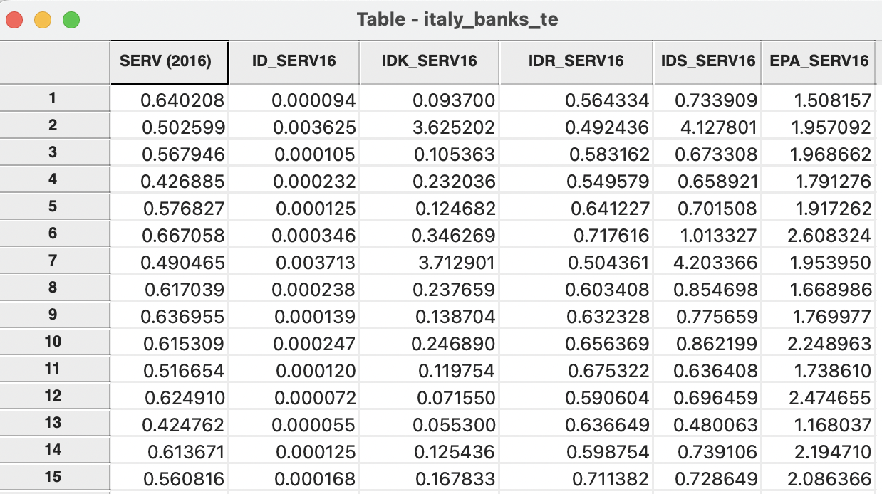
Figure 12.8: Variables computed with inverse distance weights added to table
Instead, with the inverse distances computed from coordinates in kilometers, the result in column IDK_SERV16 follow (using the weights file italy_banks_te_idk6km.gwt), essentially a rescaled version of ID_SERV16.
For example, for observation with idd=1, the inverse distance weights are given in the right-hand panel of Figure 12.2. Combining these weights with the observation values for the neighbors listed in Section 12.3.1.1 yields the value 0.093700 given in the first row of the IDK_SERV16 column.
12.3.2.2 Row-standardized inverse distance weights
The original inverse distance weights are highly scale dependent. This can be remedied by expressing them in row-standardized form. The spatial lag then takes on the standard meaning of a weighted average of the values at neighboring observations. The main difference with lags computed for connectivity weights is that now the neighbors are weighted differently. In contrast, for the straightforward spatial lag calculation of Section 12.3.1.1, all the neighboring values get the same weight.
The result of applying the row-standardized inverse distance weights from the right-hand panel in Figure 12.2 yields 0.564334, listed on the first row of the IDR_SERV16 column. In contrast to the calculation for the unstandardized inverse weights, the result is now similar in scale to the original variable (and similar to the spatial lags based on connectivity weights).
12.3.2.3 Spatial window inverse distance sum
Similar to the operations in Section 12.3.1.4, the inverse distance spatial lag can be computed for all observations in a spatial window. This is accomplished by checking the Include diagonal of weights matrix option.
However, unlike what is the case for the simple spatial lag, there is a complication on how to deal with the diagonal value. In the simple spatial lag calculation this value is either added to the neighboring observations, or averaged with them. In the inverse distance case, the neighbors are weighted, but it is not obvious what the weight should be for the diagonal, since a distance of zero does not result in a valid weight.
The convention taken in GeoDa is to keep the diagonal value unweighted. For example,
without row-standardization, this amounts to:
\[[Wy]_i = y_i + \sum_j \frac{y_j}{d_{ij}^\alpha}.\]
Again, this can be implemented in combination with a specific bandwidth for the distance.
In some contexts, this may be the desired result, but it is by no means the most intuitive concept. It should therefore be used sparingly and only when there is a strong substantive motivation. The corresponding result is listed in the first row of the IDS_SERV16 column. It is simply the sum of the value for SERV (2016) and IDK_SERV16.
The same problem occurs when using row-standardized weights. Again, in GeoDa the diagonal is unweighted, which yields:
\[[Wy]_i = y_i + \sum_j w_{ij} y_j.\]
where \(w_{ij}\) are the row-standardized inverse distance weights.
12.3.3 Using kernel weights
Spatially lagged variables can also be computed from kernel weights. However, in this instance, only one of the options with respect to row-standardization and diagonal weights makes sense. Since the kernel weights are the result of a specific kernel function, they should not be altered. Also, each kernel function results in a specific value for the diagonal element, which should not be changed. As a result, the only viable option to create spatially lagged variables based on kernel weights is to have no row-standardization and to have the diagonal elements included. Other options are not available in the interface.
Kernel-based spatially lagged variables correspond to a form of local smoothing. They can be used in specialized regression specifications, such as geographically weighted regression. The resulting spatially lagged variable is \[[Wy]_i = \sum_j K_{ij} y_j,\] When kernel weights are used, the concept of a bandwidth is already implemented in the calculation of the kernel.
For the example using Epanechnikov weights with 6 nearest neighbors (italy_banks_te_epa.kwt), the result is listed on the first row of the column EPA_SERV16. The value of 1.508157 can be obtained by combining the weights in the right-hand panel of Figure 12.5 with the neighboring observations from Section 12.3.1.1).
Creating spatially lagged variables and their use in spatial rate smoothing are the only operations in GeoDa where kernel weights can be applied. They are not available for the analysis of spatial autocorrelation.
The statistics can be readily obtained from a box plot of each variable.↩︎
The correlation can be calculated wit h the Data > View Standardized Data in a scatter plot of SERV (2016) on W1_SERV16.↩︎
The concept of population potential goes back to the early literature in social physics, e.g., Stewart (1947). See also C. Harris (1954) and Isard (1960) for extensive early discussions.↩︎