20.3 DBSCAN
The DBSCAN algorithm was originally outlined in Ester et al. (1996) and Sander et al. (1998), and was more recently elaborated upon in Gan and Tao (2017) and Schubert et al. (2017). Its logic is similar to that just outlined for the uniform kernel. In essence, the method again consists of placing circles of a given radius on each point in turn, and identifying those groupings of points where a lot of locations are within each others range.
20.3.1 Important Concepts
The DBSCAN algorithm introduces some specialized terminology to characterize the connections between points as well as the ensuing network structure.
20.3.1.1 Core, Border and Noise points
Points are classified as Core, Border or Noise depending on how many other points are within a critical distance band, the so-called Eps neighborhood. To visualize this, Figure 20.4 contains nine points, each with a circle centered on it with radius equal to Eps.127 Note that in DBSCAN, any distance metric can be used, not just Euclidean distance as in this illustration.

Figure 20.4: DBSCAN Core, Border and Noise points
A second critical concept is the number of points that need to be included in the distance band in order for the spatial distribution of points to be considered as dense. This is the so-called minimum number of points, or MinPts criterion. In the example, this is set to four. However, in contrast to the convention used before in defining k-nearest neighbors (Section 11.3.2), the MinPts criterion includes the point itself. So a MinPts = 4 corresponds to a point having 3 neighbors within the Eps radius .128
In Figure 20.4, all red points with associated red circles have at least four points within the critical range (including the central point). They are labeled as Core points (the letter C in the graph) and are included in the cluster (connected by the dashed blue lines).
The points in magenta (labeled B), with associated magenta circles have some points within the distance range (one, to be precise), but not sufficient to meet the MinPts criterion. They are potential Border points and may or may not be included in the cluster.
Finally, the blue point (labeled N) with associated blue circle does not have any points within the critical range and is labeled Noise. Such a point cannot become part of any cluster.
20.3.1.2 Reachability
A point is directly density reachable from another point if it belongs to the Eps neighborhood of that point and is one of MinPts neighbors of that point. This is not a symmetric relationship.
In the example, any red point C is directly density reachable from at least two other red points. Any such point pairs are within each others critical range. However, for border points B, the relationship only holds in one direction, as shown by the arrow. They are directly density reachable from a neighbor C, but since the B points only have one neighbor, their range does not meet the minimum criterion. Therefore, the neighbor C is not directly density reachable from B.
A chain of points in which each point is directly density reachable from the previous one is called density reachable. In order to be included, each point in the chain has to have at least MinPts neighbors and could serve as the core of a cluster. All the points labeled C in the figure are density reachable, highlighted by the dashed connections between them.
In order to decide whether a border point should be included in a cluster, the concept of density connected is introduced. A point becomes density connected if it is connected to a density reachable point. For example, the points B are each within range of a point C that is itself density reachable. As a result, the Border points B become included in the cluster.
20.3.2 DBSCAN Algorithm
In DBSCAN, a cluster is defined as a collection of points that are density connected and maximize the density reachability. The algorithm starts by randomly selecting a point and determining whether it can be classified as Core – with at least MinPts in its Eps neighborhood – or instead as Border or Noise. A Border point can later be included in a cluster if it is density connected to another Core point. It is then assigned the cluster label of the core point and no longer further considered. One implication of this aspect of the algorithm is that once a Border point is assigned a cluster label, it cannot be assigned to a different cluster, even though it might actually be closer to the corresponding core point. In a later version, labeled DBSCAN* (considered in Section 20.4), the notion of border points is dropped, and only Core points are considered to form clusters.
The algorithm systematically moves through all the points in the data set and assesses their range. The search for neighbors is facilitated by using an efficient spatial data structure, such as an R* tree. When two clusters are density connected, they are merged. The process continues until all points have been evaluated.
Two critical parameters in the DBSCAN algorithm are the distance range and the minimum number of neighbors. In addition, sometimes a tolerance for noise points is specified as well. The latter constitute zones of low density that are not deemed to be interesting.
In order to avoid any noise points, the critical distance must be large enough so that every point is at least density connected. An analogy is the specification of a max-min distance band in the creation of spatial weights, which ensures that each point has at least one neighbor. In practice, this is typically not desirable, but in some implementations a maximum percentage of noise points can be set to avoid too many low density areas.129
Ester et al. (1996) recommend that MinPts be set at 4 and the critical distance adjusted accordingly to make sure that sufficient observations can be classified as Core. As in other cluster methods, some trial and error is typically necessary. Having to find a proper value for Eps is often considered a major drawback of the DBSCAN algorithm.
20.3.2.1 Illustration
To illustrate how the DBSCAN proceeds, a toy example of nine points is depicted in Figure 20.5. The inter-point distances are included on the graph. The typical point of departure is to consider a connectivity structure that ensures that each point has at least one neighbor, i.e., the max-min critical distance. In the example, this distance is 29.1548, with the corresponding number of neighbors in the connectivity graph ranging from 1 to 5.
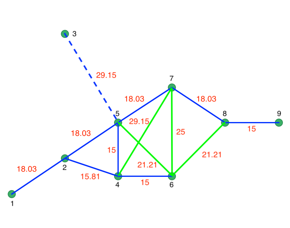
Figure 20.5: Connectivity graph for Eps = 20
The concept of Noise points (i.e., unconnected points for a given critical distance) becomes clear when the Eps distance is set to 20. In Figure 20.5, this results in one unconnected point, labeled 3, shown by the dashed blue line between 3 and 5. The green lines correspond with inter-point distances that do not meet the Eps criterion either, but they do not result in isolates. The effective connectivity graph for Eps = 20 is shown in solid blue.
With MinPts as 4 (i.e., 3 neighbors for a core point), the algorithm proceeds through each point, one at a time. For example, it could start with point 1, which only has one neighbor (point 2) and thus does not meet the MinPts criterion. Therefore, it is initially labeled as Noise. Next, point 2 is considered. It has 3 neighbors, meaning that it meets the Core criterion, and therefore it is labeled cluster 1. All its neighbors, i.e., 1, 4 and 5 are also labeled cluster 1 and are no longer considered. Note that this changes the status of point 1 from Noise to Border. Point 3 has no neighbors and is therefore labeled Noise.
Next is point 6, which is a neighbor of point 4 that belongs to cluster 1. Since 6 is therefore density connected, it is added to cluster 1 as a Border point. The same holds for point 7, which is similarly added to cluster 1.
Point 8 has two neighbors, which is insufficient to reach the MinPts criterion. Even though it is connected to point 7, which belongs to the cluster, 7 is not a Core point, so therefore 8 is not density connected and is labeled Noise. Finally, point 9 has only point 8 as neighbor and is therefore labeled Noise as well.
This results in one cluster consisting of 6 points, shown as the dark blue points in Figure 20.6. The solid blue lines show the connections between the Core points, the dashed lines show the Border points. The light blue points for 3, 8 and 9 indicate Noise points.
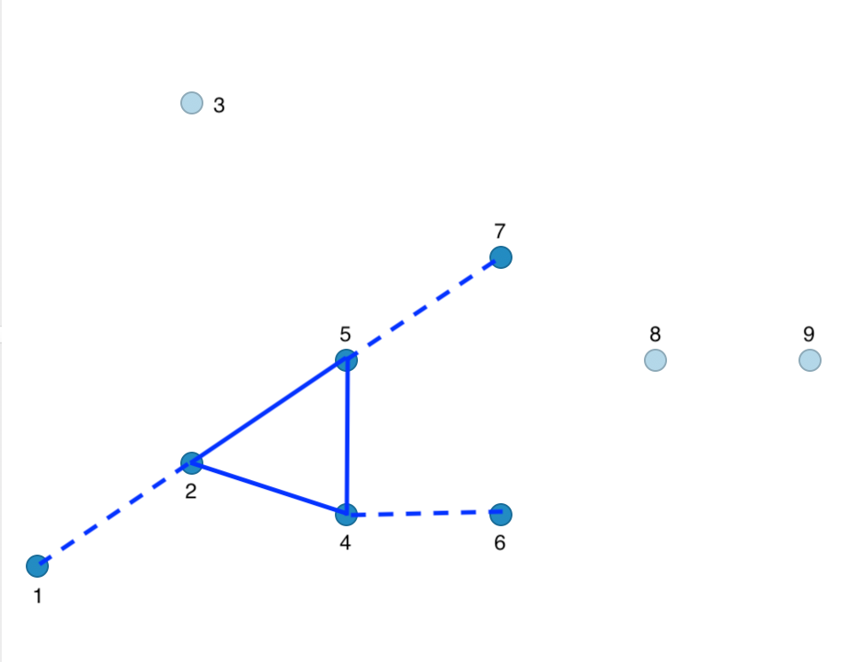
Figure 20.6: DBSCAN clusters for Eps = 20 and MinPts = 4
20.3.3 Implementation
DBSCAN is invoked from the cluster toolbar icon (Figure 20.1) as the first item in the density cluster group, or from the menu as Clusters > DBScan . This brings up the DBScan Clustering Settings dialog, which combines two functions. One is the specification of variables and various cluster options, shown in the left-hand panel of Figure 20.7. The other is the presentation of Summary characteristics of the resulting clusters, and, for DBSCAN*, the Dendrogram (see Section 20.4.2.1).
The Select Variables panel includes the variables that must be chosen as X and Y coordinates. For the Italy Community Banks sample data set, the variables XKM and YKM are specified, which correspond with the projected coordinates expressed in kilometers (the original is in meters). The selected Method is DBScan.
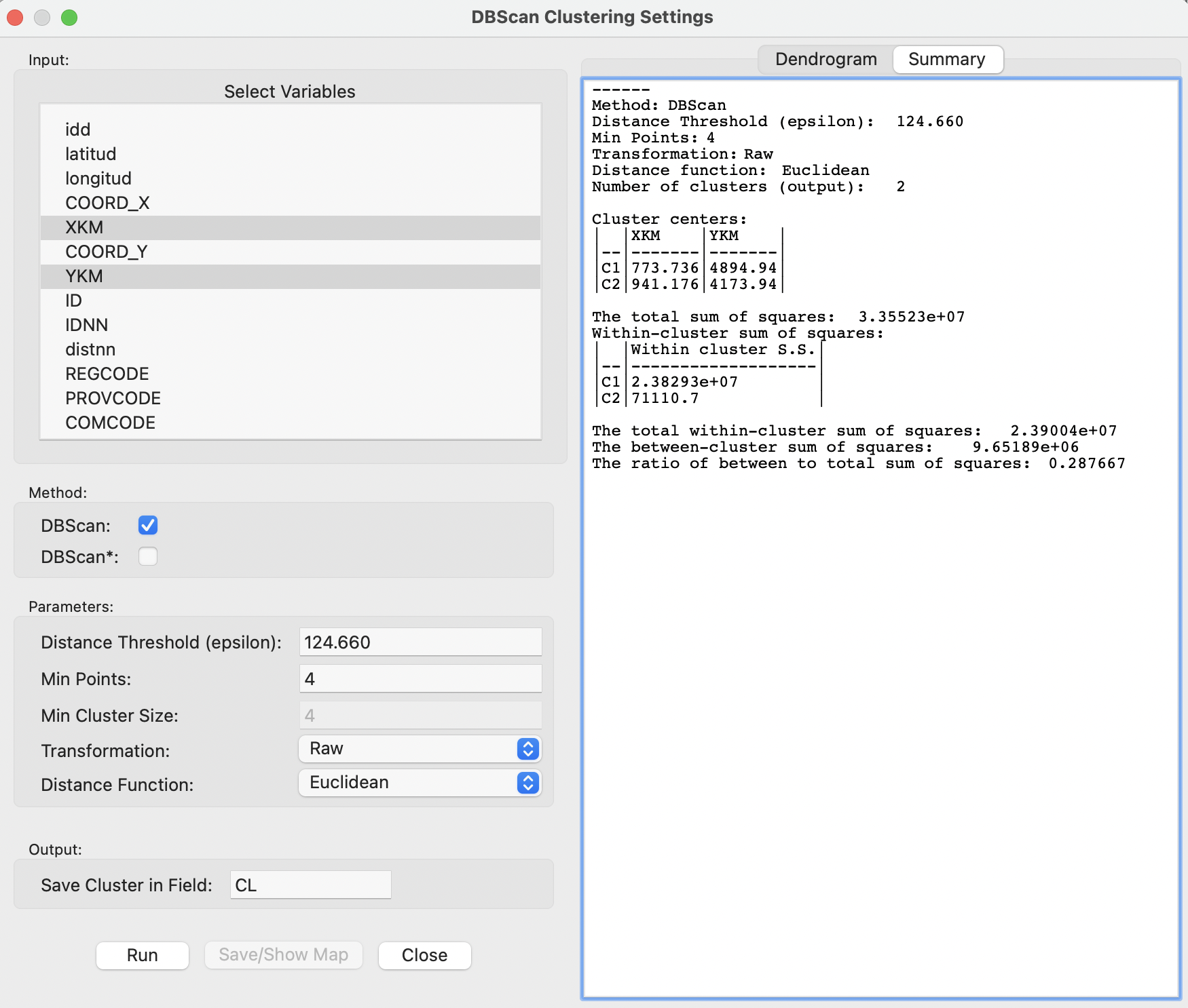
Figure 20.7: DBSCAN Clustering Settings
The selection of the coordinates immediately populates some of the fields in the Parameters panel. The default Transformation is Standardize (Z), with the Distance Threshold (epsilon) as 0.443177. However, in this instance, the original coordinates should be used, hence the Raw option is specified in Figure 20.7. This yields a critical distance of 124.659981. As it turns out, a slight correction is needed, and the value is rounded to 124.660 in the dialog.
The other options consist of the Min Points, which is initially left to the default of 4, and the Distance Function, set to Euclidean (the other option is Manhattan distance). The Min Cluster Size option is not available for DBSCAN.
A final item to be specified is the variable that will contain the cluster identifier (Save Cluster in Field), with CL as the default. In GeoDa the identifiers are assigned in decreasing order of the size of the cluster, i.e., with 1 for the largest cluster. Points that remain as Noise points are assigned a value of 0.
20.3.3.1 Cluster map and summary
The resulting cluster map for the default settings is shown in Figure 20.8. Only two clusters are identified, one very large one, consisting of 242 bank locations on the mainland, the other, a very small one of 19 banks on the island of Sicily. Given the choice of the max-min bandwidth, there are no Noise points.
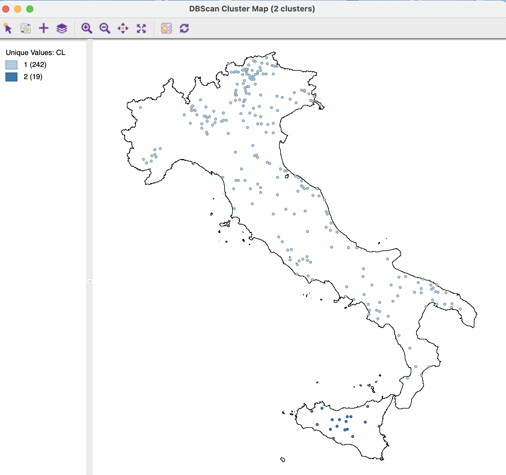
Figure 20.8: Default DBSCAN Cluster Map
The Summary in the right-hand panel of Figure 20.7 lists the parameters used, the cluster centers and within-cluster sum of squares, as well as an overall summary of the fit, the ratio of between to total sum of squares. The value of 0.288 is very low, which is not surprising, given the large number of points contained in the main cluster, which results in a high within-cluster sum of squares. The specifics of these summary measures are discussed in more detail in the treatment of spatial clustering in Volume 2.
20.3.3.2 Sensitivity analysis
In most applications, the default parameters are just a point of departure and considerable sensitivity analysis is needed to assess the effect of changes in the settings. Specifically, the two main parameters of Distance Threshold and Min Points play a crucial role. As an illustration, the results of a cluster analysis with a bandwidth of 50km and the minimum points set to 10 are given in Figure 20.9. In addition to the cluster points, identified by different colors, the connectivity graph for a 50km distance band is shown as well. Seven clusters are identified, ranging in size from 110 to 10 observations. A total of 70 locations are labeled Noise, either because they become isolates (not connected to the graph), or they have insufficient neighbors. The overall fit of the clusters is much better, with a between to total ratio of 0.957 (not shown), due to a grouping of locations that are relatively close by.
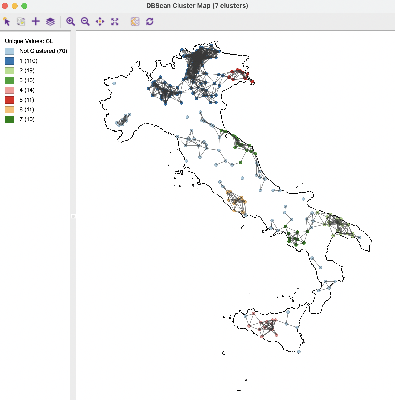
Figure 20.9: DBSCAN Cluster Map, Eps=50, Min Pts=10
20.3.3.3 Border points and minimum points
In some instances, the outcome of a DBSCAN algorithm can lead to seemingly counter intuitive results. For example, using the Italian bank data with a 50km bandwidth and 8 minimum points yields 10 clusters and a good fit of 0.960. However, cluster 10 consists of only 6 observations, less than the minimum points requirement (results not shown). This is a result of the peculiar way in which Border points are treated. Specifically, as mentioned above, they are assigned to the first set of density reachable points to which it is density connected, even though it may be closer to a later cluster. The specific implementation of the algorithm does not change the allocation, but does recognize the later clusters as such, even with less than minimum points.
The figure is loosely based on Figure 1 in Schubert et al. (2017).↩︎
This definition of MinPts is from the original paper. In some software implementations, the minimum points pertain to the number of nearest neighbors, i.e., MinPts - 1.
GeoDafollows the definition from the original papers.↩︎GeoDacurrently does not support this option.↩︎