19.5 Quantile LISA
The Local Join Count statistics are designed to deal with binary variables. The principles behind these statistics can be readily extended to the situation where a subset of observations on a continuous variable is selected based on a specific value interval. The most straightforward example is when all the observations in a given quantile are assigned a value of 1, and the remaining observations become 0. As a result, assessing local spatial autocorrelation in this case can be approached as an extension of the Local Join Count statistics.
In Anselin (2019b), this case is referred to as Quantile LISA or quantile local spatial autocorrelation. In a bivariate or multivariate setting, the quantile LISA often serves as a viable alternative to a Bivariate Local Moran or a Multivariate Local Geary, especially when the focus is on extremes in the distribution.
As discussed in Section 18.3, the continuous (linear) association between two variables that is measured by the Bivariate Local Moran suffers from the problem of in-situ correlation. The quantile local spatial autocorrelation sidesteps this problem by converting the continuous variable to a binary variable that takes the value of 1 for a specific quantile. By considering either co-location (positive in-situ correlation) or no co-location (negative in-situ correlation), the correlation between the two variables can be controlled for.
For example, the spatial association between two continuous variables can be simplified by focusing on the local autocorrelation between binary variables for the upper quintile. Since the bivariate (or multivariate) Local Join Count statistic enforces co-location, the problem of in-situ correlation is controlled for. This provides an alternative to other bivariate and multivariate local spatial autocorrelation statistics, albeit with a loss of information, associated with going from the continuous variable to a binary category.
In addition, the quantile LISA approach can also be employed to assess negative spatial autocorrelation, such as between the upper and lower quantile of the same variable. This becomes a special case of a No-Colocation Bivariate Local Join Count statistic.
The quantile approach focuses on a subset of a distribution and thus constitutes a loss of information. However, in practice, this loss of information is often compensated for by superior insight and a focus on the most important interesting locations.
Formally, a continuous variable \(y\) with a cumulative density function \(F(y)\) yields a sequence of ranked observations as \(y_1, y_2, \dots, y_n\). A new binary variable \(x\) is created that takes on the value \(x_i = 1\) for all \(y_i\) for which \[y_{ql} \le y_i < y_{qu},\] with \(y_{ql}\) and \(y_{qu}\) as lower and upper bounds for a given quantile.125 For all other observations, \(x_i = 0\).
The new \(x\) variable (or set of such variables in a multivariate case) then forms the basis for analysis by means of a Local Join Count statistic, or one of its multivariate extensions.
19.5.1 Implementation
The Univariate and Multivariate Quantile LISA are invoked from the next to last block in the drop down list associated with Cluster Maps icon on the toolbar, or, from the menu, as Space > Univariate Quantile LISA and Space > Multivariate Quantile LISA respectively.
The Quantile LISA Dialog contains several options. In the univariate case, the continuous variable needs to be specified, together with the spatial weights. Next follow the criteria to create the binary form of the variable: the Number of Quantiles, Select a Quantile for LISA, and Save Quantile Selection in Field. The default number of quantiles is 5, for quintiles. The quantile selection consists of a drop down list with appropriate values, i.e., in this example 1 to 5, with 1 for the lowest quantile (in this case, quintile), and 5 for the highest. The resulting binary variables is added to the data table with a default variable name of QT.
In the multivariate case, a similar interface allows for the creation of one binary variable at a time, with for each the number of categories and the order of the selected category, saved under default variables QTk, with k as the sequence number. Each newly created variable must be moved to the right-hand panel of the dialog by means of the > button (and, conversely, can be removed by means of the < button).
A check box determines whether No co-location must be enforced. The default is to allow co-location. A warning message results in case of no overlap when there should be overlap, and vice versa.
With the spatial weights selected, the analysis is run and a significance map is created. This is illustrated with three specific cases: a univariate Quantile LISA, and a bivariate and multivariate example. All the standard options are available.
19.5.2 Univariate Quantile LISA
To illustrate the univariate Quantile LISA case, consider the upper quintile of the variable ChldPvt14, the children poverty rate. A quartile map (but not a quintile map) was shown earlier in Figure 18.1. The upper quintile is converted into a binary variable ChildPvt5, shown in the unique values map in the left-hand panel of Figure 19.6.
The right-hand panel shows the significance map using 99,999 permutations with a p-value cut-off of 0.05, for queen contiguity (Chi_SDOH_q). The highlighted locations form a subset of the cores identified by means of the Local Moran map in the left-hand panel of Figure 18.3. Of the 101 High-High cluster cores at p=0.01 in the Local Moran cluster map, 61 are retained in the Quantile LISA significance map. Three of these are highly significant at p=0.00001.
Obviously, Low-Low clusters and spatial outliers are not considered. Nevertheless, the Quantile LISA approach identifies essentially the same interesting High-High cluster locations as the analysis that uses the full continuous distribution.
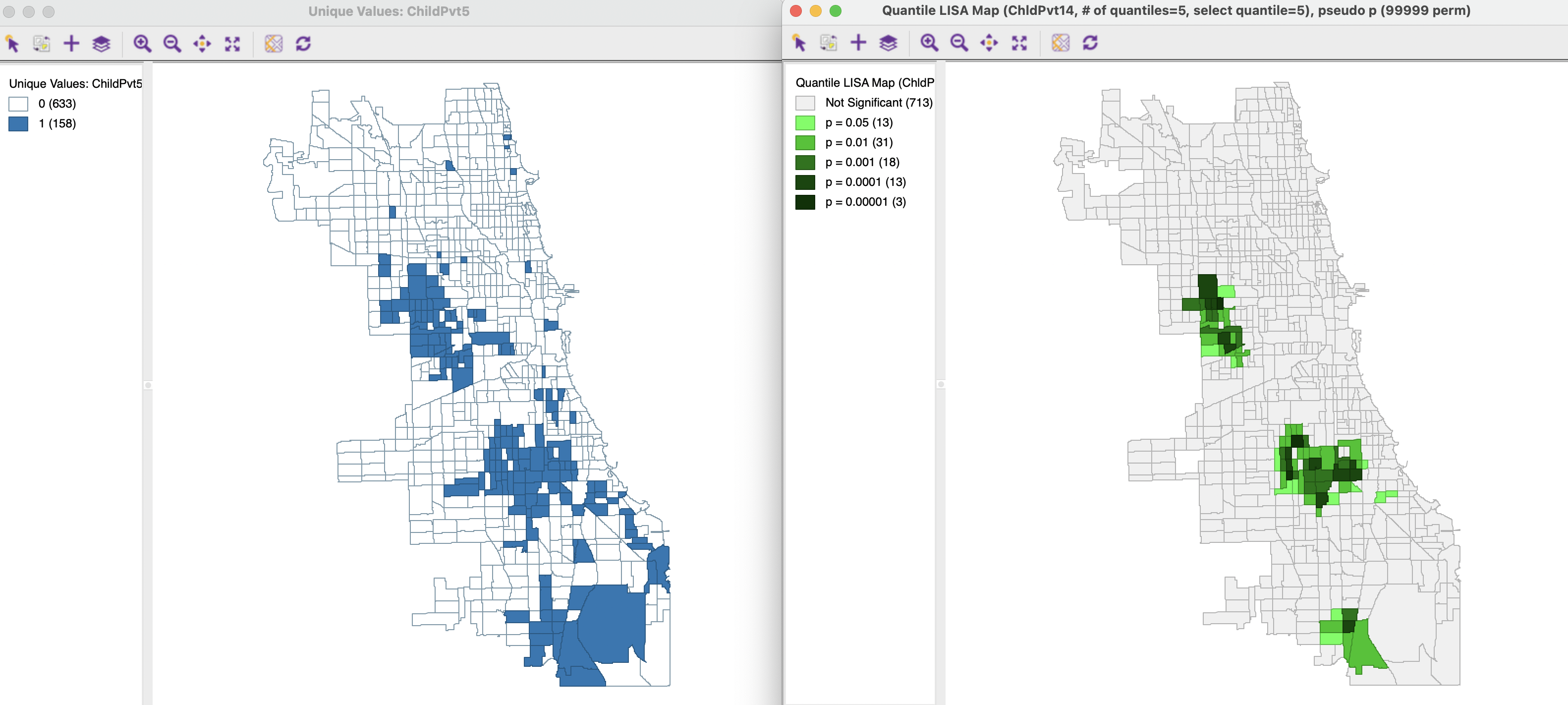
Figure 19.6: Univariate Quantile LISA
19.5.3 Bivariate and Multivariate Quantile LISA
The bivariate case allows for both no co-location (box checked) and co-location, as specified through the Multivariate Quantile LISA Dialog. The No co-location option only works in the bivariate case and provides a way to address negative spatial autocorrelation, i.e., spatial outliers. For example, this can be used to assess whether observations in a top quantile are surrounded by locations in a bottom quantile, or vice versa (as pointed out, the statistic is not symmetric).
The co-location option is the default and it allows to identify clusters of observations that belong to specified quantiles for different variables. Typically, this will be the top or bottom quantiles, but the tool is sufficiently flexible to allow any combination (provided it makes sense). A critical constraint is that there need to be co-location of the quantiles for all the variables considered. For example, if three variables are taken into account, then there must be locations (at least one), where the respective quantiles coincide. Just as for the multivariate local join count, this becomes harder to satisfy as more variables are being considered.
19.5.3.1 Spatial Outliers
The No co-location option is illustrated in Figure 19.7 for the lower and upper quintiles of the variable ChldPvt14, using 99,999 permutations with p = 0.05 and queen contiguity spatial weights. Only one census tract can be identified that belongs to a bottom quintile and is surrounded by more neighbors from the top quintile than likely under spatial randomness. Moreover, the evidence is very weak and only holds for p = 0.05. Note that the same location was also identified as a Low-High spatial outlier in the Local Moran cluster map in Figure 18.3.
The reverse assessment, for top quintiles surrounded by bottom quintiles, does not yield a single significant location.
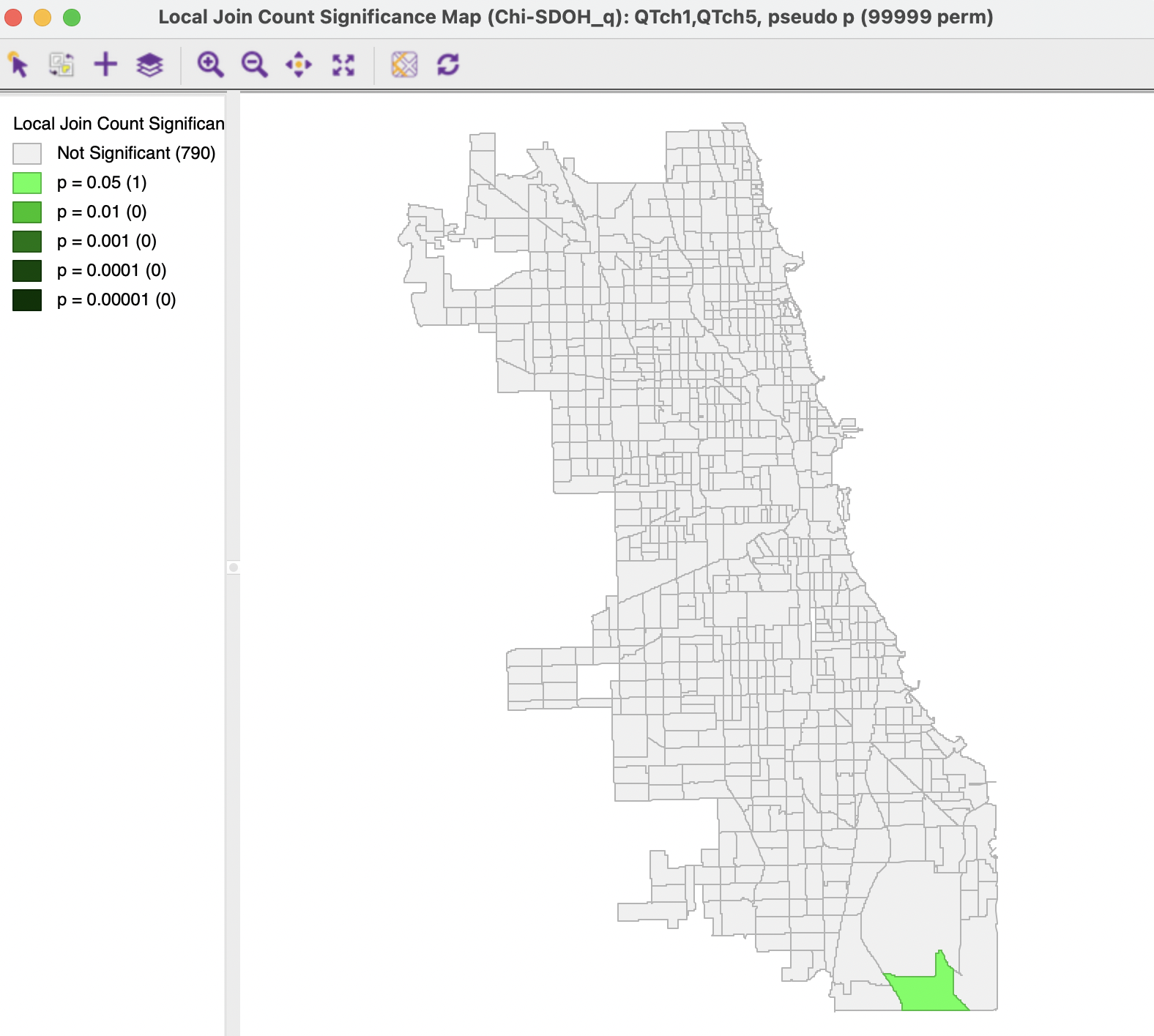
Figure 19.7: Spatial Outliers with Quantile LISA
19.5.3.2 Multivariate Co-Location
The multivariate co-location case is illustrated with the same three variables as used for the Multivariate Local Geary in Section 18.4.1, but now for queen contiguity spatial weights. The three variables, child poverty (ChldPvt14), crowded housing (EP_CROWD), and lack of health insurance (EP_UNINSUR) are converted into indicator variables with a value of 1 for those observations belonging to the top quintile. The corresponding Multivariate Quantile LISA significance map is shown in the left-hand panel of Figure 19.8, for 99,999 permutations and p = 0.05.
Eight cluster cores are identified, of which three at p = 0.001. The cluster map on the right shows the significant locations for the corresponding Multivariate Local Geary (using the Bonferroni bound for 0.01 and 99,999 permutations). The Multivariate Local Geary cluster map includes 35 cluster cores. Of those, only two are also identified by the Multivariate Quantile LISA. The six others, are not found to be significant in the Multivariate Local Geary cluster map.
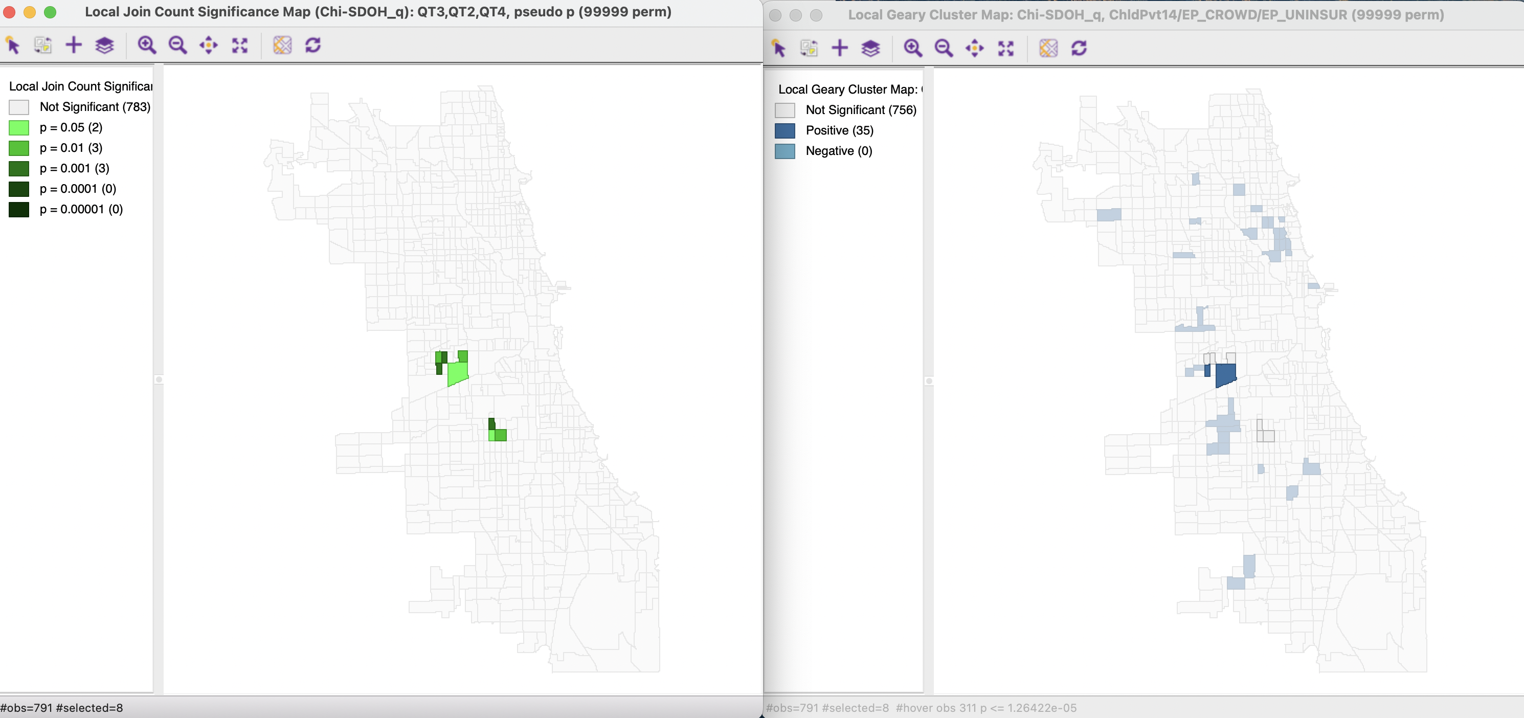
Figure 19.8: Multivariate Quantile LISA and Multivariate Local Geary
In contrast to the large number of significant locations obtained with the Multivariate Local Geary, the Quantile version focuses on a much smaller (sub)set of significant observations and may thus provide clearer insight into the interesting locations.
In general, this may be applied to any interval, not just a given quantile.↩︎