2.2 Spatial Data

Spatial data are characterized by the combination of two important aspects. First, there is information on variables, just as in any other statistical analysis. In the spatial world, this is referred to as attribute information. Typically, it is contained in a flat (rectangular) table with observations as rows and variables as columns.

The second aspect of spatial data is special, and is referred to as locational information. It consists of the precise definition of spatial objects, classified as points, lines or areas (polygons). In essence, the formal characterization of any spatial object boils down to the description of X-Y coordinates of points in space, as well as of a mechanism that spells out how these points are combined into spatial entities.

For a single point, the description simply consists of its coordinates. For areal units, such as census tracts, counties, or states, the associated polygon boundary is defined as a series of line segments, each characterized by the coordinates of their starting and ending points. In other words, what may seem like a continuous boundary, is turned into discrete segments.

Traditional data tables have no problem including X and Y coordinates as columns, but as such cannot deal with the boundary definition of irregular spatial units. Since the number of line segments defining an areal boundary can easily vary from observation to observation, there is no efficient way to include this in a fixed number of columns of a flat table. Consequently, a specialized data structure is required, typically contained in a geographic information system or GIS.

Several specialized formats have been developed to efficiently combine both the attribute information and the locational information. Such spatial data can be contained in files with a special structure, or in spatially enabled relational data base systems.

I first consider common GIS file formats that can serve as input to GeoDa. This is followed by an illustration of simple tabular input of non-spatial files. Finally, a brief overview is given of connections to other input formats.

2.2.1 GIS files

Historically, a wide range of different formats have been developed for GIS data, both proprietary as well as open source. In addition, there has been considerable effort at standardization, led by the Open Geospatial Consortium (OGC).¹ GeoDa leverages the open source GDAL library² to support input and output of many of the most popular formats in use today.

While it is impossible to cover all of these specifications in detail, I will illustrate three specific formats here. First is the use of the proprietary shape file format of the leading GIS vendor ESRI.³ In addition, the open source GeoJSON format⁴ will be covered, as well as the Geography Markup Language of the OGC, a standard XML grammar for defining geographical features.⁵

In GeoDa, one can load both polygon and point GIS data, but in the current implementation, line files are not supported (e.g., to represent road networks).

2.2.1.1 Spatial file formats

Arguably, the most familiar proprietary spatial data format is the shape file format, developed by ESRI. The terminology is a bit confusing, since there is no such thing as one shape file, but there is instead a collection of three (or four) files. One file has the extension .shp, one .shx, one .dbf, and one .prj (with the projection information). The first three are required, the fourth one is optional, but highly recommended. The files should all be in the same directory and have the same file name, except for the file extension.

In the open source world, an increasingly common format is GeoJSON, the geographic augmentation of the JSON standard, which stands from JavaScript Object Notation. This format is contained in a text file and is easy for machines to read, due to its highly structured nature.

Finally, the GML standard, or Geographic Markup Language, is a XML implementation that prescribes the formal description of geographic features.

A detailed discussion of the individual formats is beyond the current scope. All are well-documented, with many additional resources available online. Although it is always helpful, there is no need to know the underlying formats in detail in order to use GeoDa, since the interaction with the data structures is handled under the hood.

The main file manipulations are invoked from the File item in the menu, or by the three left-most icons on the toolbar in Figure 2.1.

2.2.1.2 Polygon layers

Since GeoDa is particularly geared to the exploration of areal unit data, the input of a so-called polygon layer is illustrated first. Any spatial layer present as a file can be loaded by invoking File > Open File from the menu, or by clicking on the left-most Open icon on the toolbar in Figure 2.1.

This brings up the Connect to Data Source dialog, shown in Figure 2.2. The left panel has File as the active input format. Other formats are Database and Web, which are briefly covered in Section 2.2.3. The right panel shows a series of Sample Data data that are included with GeoDa. In addition, after some files have been loaded in the current application, the Recent panel will contain their file names as well. Files listed in either panel can be loaded by simply clicking on the corresponding icon.

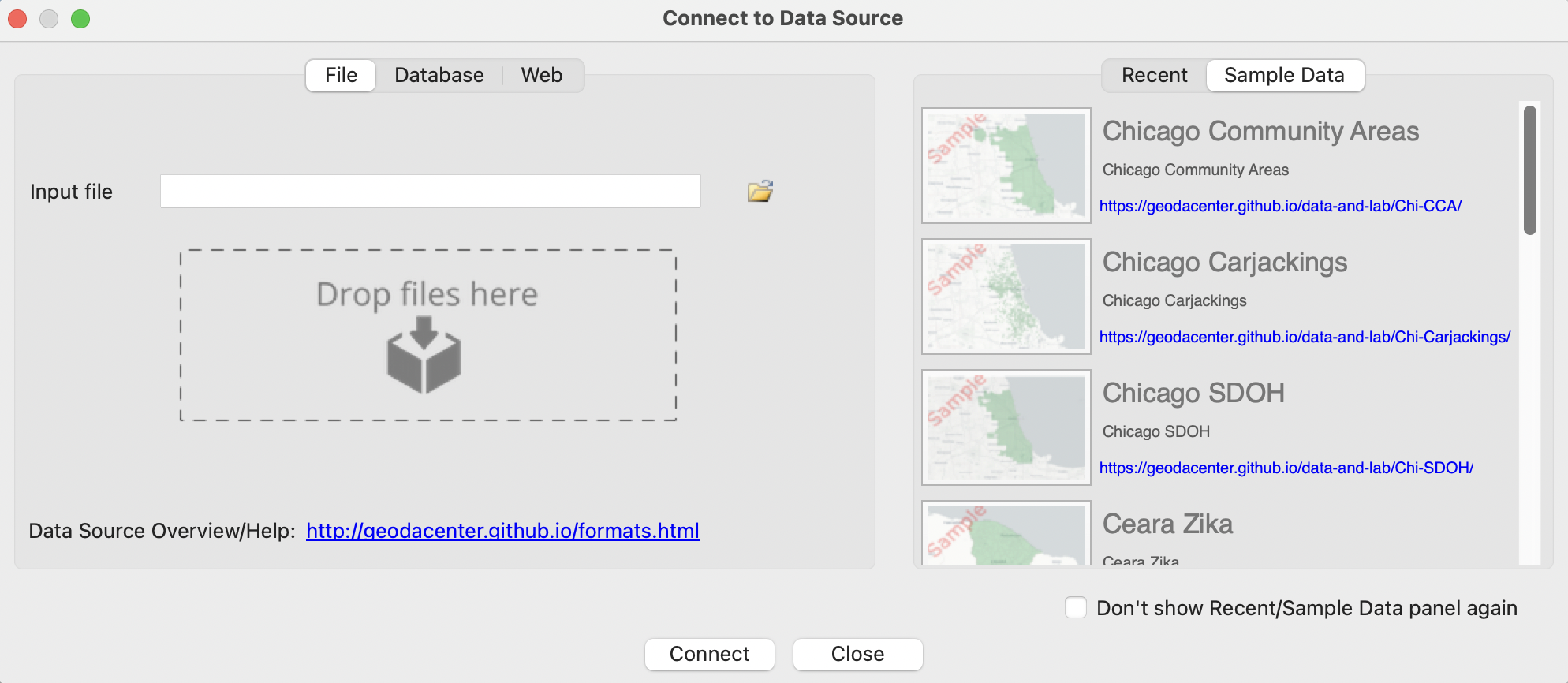
Figure 2.2: Connect to Data Source dialog

The small folder icon to the right of the Input file box brings up a list of supported file formats, as in Figure 2.3. In this first example, the top item in the list is selected, ESRI Shapefile (*.shp).

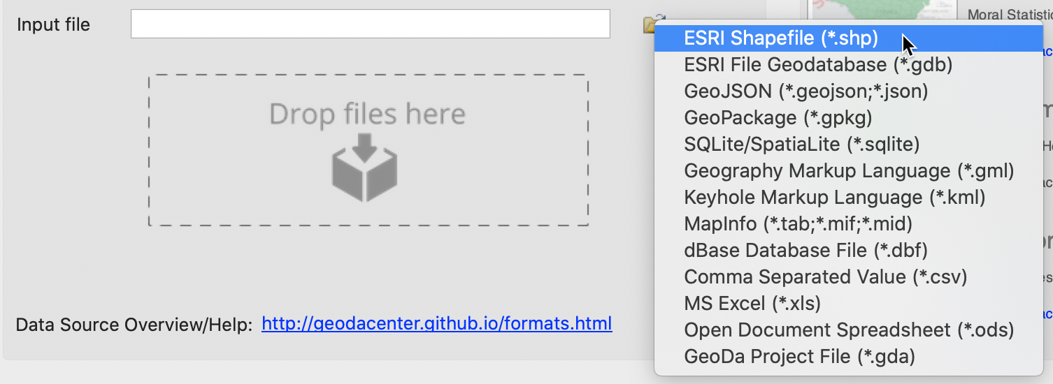
Figure 2.3: Supported spatial file formats

To illustrate this feature, the four files associated with the Chicago_community_areas shape file must be available in a working directory (they must be downloaded from the GeoDaCenter sample data site).

Using the navigation dialog and conventions appropriate for each operating system, the shape file can be selected from this directory. This opens a new map window with the spatial layer represented as a themeless choropleth map, as in Figure 2.4. The number of observations is shown in parentheses next to the small green rectangle in the upper-left panel, as well as in the status bar at the bottom (#obs = 77).

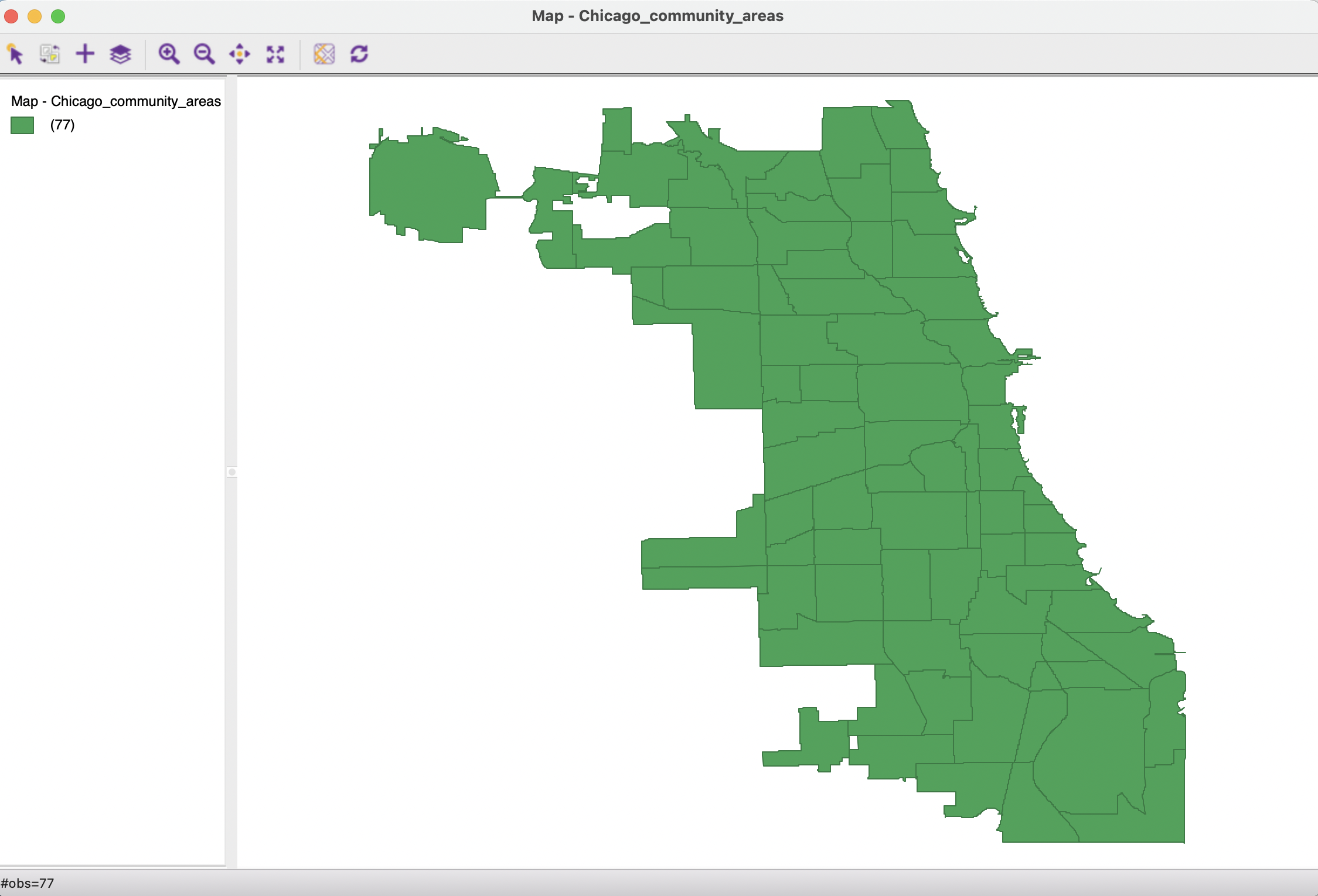
Figure 2.4: Themeless polygon map

The current layer is cleared by clicking on the Close toolbar icon, the second item on the left in Figure 2.1, or by selecting File > Close from the menu. This removes the base map. At this point, the Close icon on the toolbar becomes inactive.

A more efficient way to open files is to select the file name in the directory window and to drag it onto the Drop files here box in the dialog. Even easier is to load a one of the sample data sets or a recently used one, where a simple click on the associated icon in the Sample Data or Recent tab suffices.

In contrast to the shape file format, which is binary, a GeoJSON file is simple text and can easily be read by humans. As shown for the Chicago_community_areas.geojson file from the sample data site in Figure 2.5 (this file must be downloaded to a working directory), the locational information is combined with the attributes. After some header information follows a list of features. Each of these contains properties, of which the first set consists of the different variable names with the associated values, just as would be the case in any standard data table. The final item refers to the geometry. This includes the type, here a MultiPolygon, followed by a list of X-Y coordinates. In this fashion, the spatial information is integrated with the attribute information.

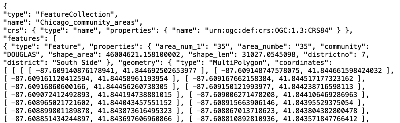
Figure 2.5: Example GeoJSON file contents

To view the corresponding map, the Chicago_community_areas.geojson file name can be selected in its directory and dragged onto the Drop files here box. This brings up the same base map as in Figure 2.4.

2.2.1.3 File format conversion

The file just loaded was originally specified in the GeoJSON format. It can be easily converted to a different format by means of the File > Save As functionality. For example, to change it into a GML format file (e.g., for use in a different program), Geographic Markup Language (*.gml) can be selected from the drop down list of available formats, shown in Figure 2.3.

With an output file name as Chicago_community_areas.gml specified in the file dialog, this will yield a text file in the GML XML format. Its contents are illustrated in Figure 2.6, showing the characteristic < > and </ > delimiters of the markup elements, typical of XML files.

In the file snippet in the figure, the top lines pertain to the geography of the first polygon, ended by </ogr:geometryProperty>. Next follow the actual observations, with variable names and associated values, finally closed off with </ogr:featureMember>. After this, a new observation is listed, delineated by the <ogr:featureMember> tag, followed by the geographic characteristics. Again, this illustrates how spatial information is combined with attribute information in an efficient file format.

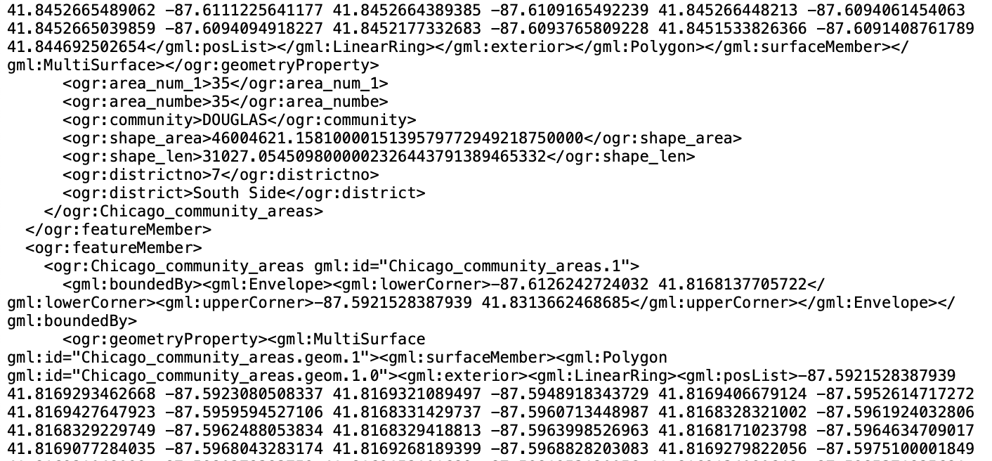
Figure 2.6: Example GML file contents

In sum, the File > Save As feature in GeoDa turns the program into an effective GIS format converter.

2.2.1.4 Point layers

In the same fashion as for polygon layers, spatial data layers containing point locations can be loaded for the file formats listed in Figure 2.3. As before, the file is either selected explicitly from the proper directory, or the file name is dragged directly into the Drop files here box in the dialog.

The point map in Figure 2.7 shows the locations of the 1,412 carjackings that occurred in the City of Chicago during the year 2020. It is generated by clicking on the Chicago Car Jackings icon in the Sample Data tab, or by dragging the file name Chicago_carjack_2020_pts.shp from a working directory that contains the shape file.

The shape of the city portrayed by the outline of the points is slightly different from that in the polygon map in Figure 2.4. This is due to a difference in projections: the point map is in the State Plane Illinois East NAD 1983 projection (EPSG 3435), whereas the polygon map uses decimal degrees latitude and longitude (EPSG 4326). This important aspect of spatial data is often a source of confusion for non-GIS specialists. GeoDa provides an intuitive interface to deal with projection issues. I return to this topic in Section 2.3.1.1 below and in Section 3.2 in the next chapter.

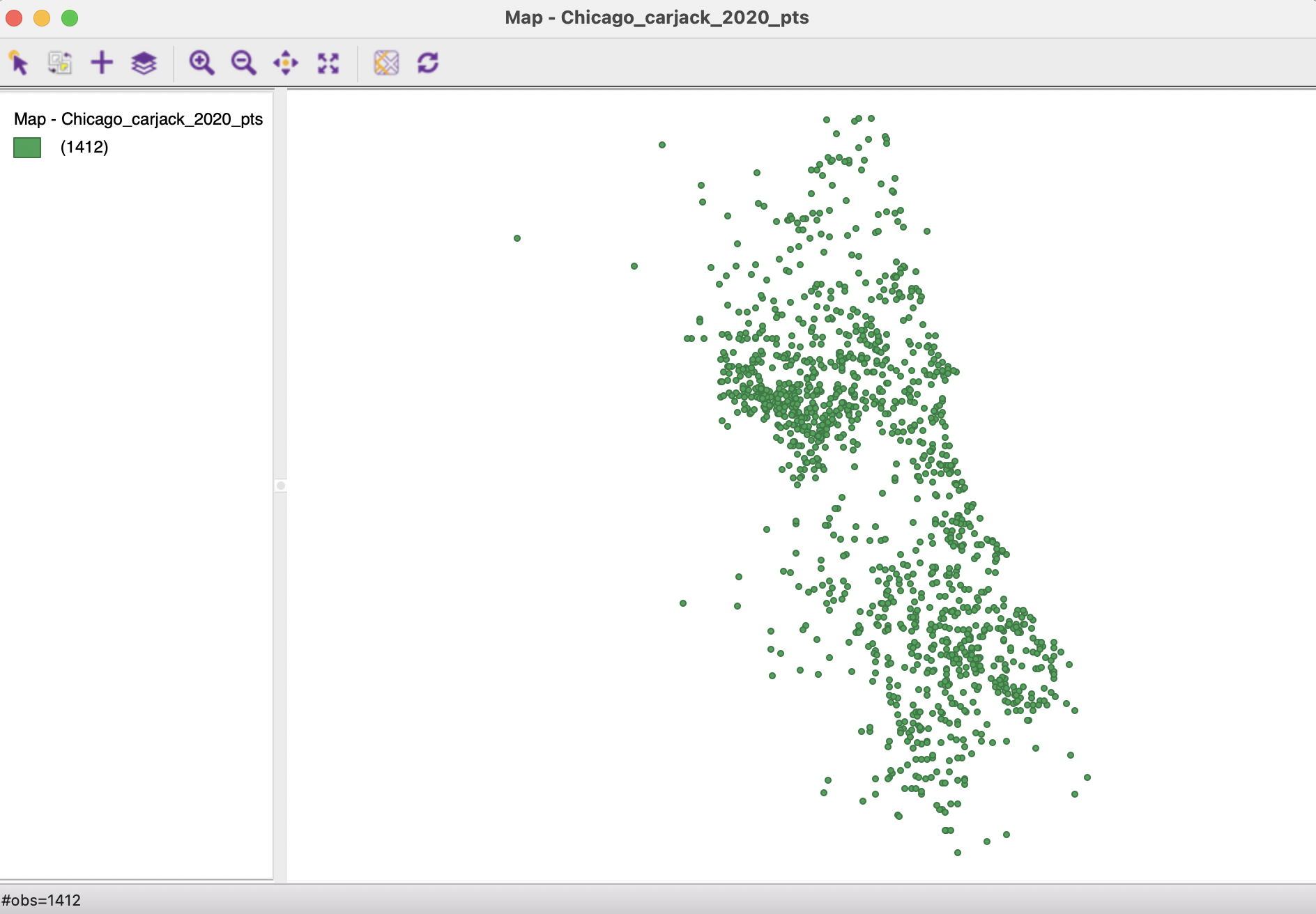
Figure 2.7: Themeless point map

2.2.2 Tabular files

In addition to GIS files, GeoDa can also read regular non-spatial tabular data. While this does not allow for spatial analysis (unless coordinates are contained in the table, see Section 2.3.1), all non-spatial operations and graphs are supported. Specifically, all standard techniques of exploratory data analysis (EDA) can be applied, as covered in Chapters 7 and 8 in this Volume. This does not necessitate a map layer.

The data for the Community area socio-economic profiles are contained in a comma separated file (csv format) on the sample data site (the Chicago CCA Profiles are also available as a spatial layer in the Sample Data tab). Selecting this file (after downloading it to a working directory) generates the dialog shown in Figure 2.8.

Since a csv file is pure text, there is no information on the type of the variables included in the file. GeoDa tries to guess the type and lists the Data Type for each field, as well as a brief preview of the table. At this point, the type can be changed before the data are moved into the actual data table (see also Section 2.4.1.1).

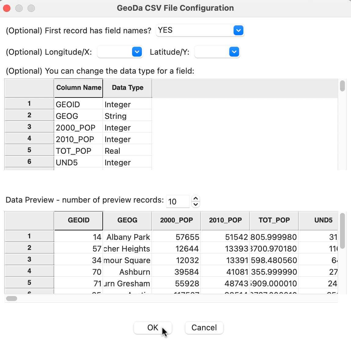
Figure 2.8: CSV format file input dialog

Instead of a base map, which is the default opening window for spatial data, the data table is brought up in a spreadsheet-like format (see also Figure 2.9 for an illustration). In addition to comma separated files, GeoDa also supports tabular input from dBase database files, Microsoft Excel, and Open Document Spreadsheet (*.ods) formatted files. As is the case for the various GIS formats, the File > Save As command allows for the ready conversion from one tabular format to another (e.g., from csv to dBase).

An additional feature of the input dialog in Figure 2.8 is inclusion of optional Longitude/X and Latitude/Y drop down lists. With coordinate variables specified, this will create a point layer. As such, it provides an alternative to the approach outlined in Section 2.3.1.

2.2.3 Other spatial data input

In addition to file input, GeoDa can connect to a number of spatially enabled relational data bases, such as PostgesQL/PostGIS, Oracle Spatial and MySQL Spatial. This is available through the Database button in the Connect to Data Source interface, the middle tab in the dialog shown in Figure 2.2. Each data base system has its own requirements in terms of specifying the host, port, user name, password and other settings. Once the connection is established, the data can also be saved to a file format. In the current version of GeoDa, the data base connection is limited to loading a single table. So far, no other SQL commands are supported.

A third data source option is referred to as Web in the interface, the right-most tab in Figure 2.2. It allows data to be loaded directly from a GeoJSON URL, or, alternatively, from the older web feature server WFS URL.