12.4 Spatial Weights in Rate Smoothing
In the discussion of rate smoothing in Chapter 6, two approaches were left until after spatial weights were introduced. Spatial rate smoothing and spatial Empirical Bayes smoothing are extensions of, respectively, the raw rate map and Empirical Bayes smoothing. The spatial versions are distinct in that they incorporate values for neighboring observations into the numerator and denominator of the rate calculation. This is made operational through the use of spatially lagged variables.
These methods will be illustrated with the municipal disability rate in 2020 from the Oaxaca Development sample data set. In addition to variables, five different spatial weights matrices will be employed: first order queen contiguity (oaxaca_q.gal); inclusive second order queen contiguity (oaxaca_q2.gal); nearest neighbor weights, with k=6 (oaxaca_k6.gwt); inverse distance weights with a 6 nearest neighbor bandwidth (oaxaca_idk6.gwt); and block weights based on the region classification (oaxaca_reg.gal).
12.4.0.1 Oaxaca disability rate
The disability rate is obtained as the ratio of the number of disabled persons (DIS20) over the population (PTOT20) in 2020.
This rate provides a prime example of variance instability (see Section 6.4.1), due to the wide range of population totals for municipalities, including several with very small values. In 2020, the municipal population for the 570 municipalities ranged from 81 to 270,955, and 47 locations had fewer than 500 inhabitants. The average population was 7,249, but the median was much smaller, at 2,881, reflecting the effect of upper outliers (there are 62 such outliers, with populations ranging from 14,198 to 270,955). This will yield substantial variation in the precision of the computed raw rates.
To provide some reference for the later illustrations, Figure 12.9 includes the raw rate map (Section 6.2.2) in the left-hand panel and the Empirical Bayes (EB) smoothed rate map (Section 6.4.2.2) in the right-hand panel.
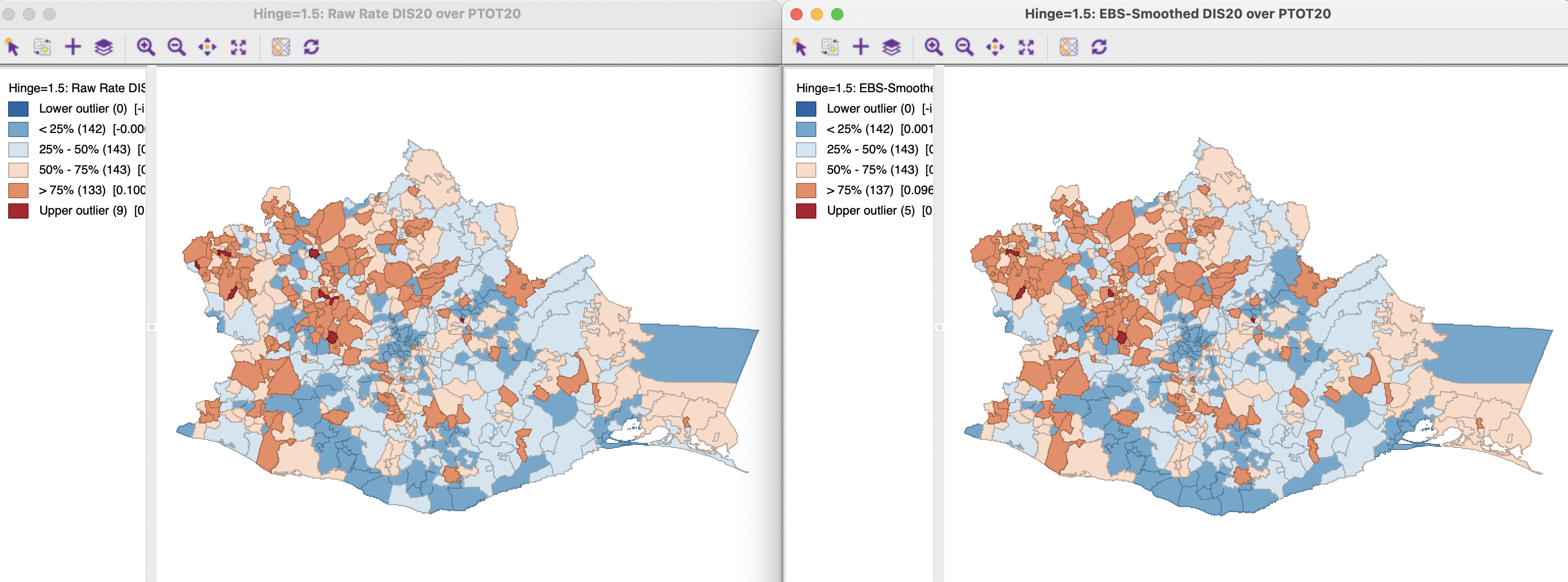
Figure 12.9: Disability rate: raw rate and EB smoothed rate
The effect of the smoothing is to eliminate a few upper outliers in the map. Otherwise, the relative ranking of observations in quartiles is not much affected. However, there is a real impact on the actual values. The range is reduced from 0.0149 to 0.3161 for the raw rate, to a much narrower 0.0174 to 0.2164 for the smoothed rate. The correlation between the two rates is 0.984.
12.4.1 Spatial rate smoothing
A spatial rate smoother is a special case of a nonparametric rate estimator, based on the principle of locally weighted estimation (see, e.g., Waller and Gotway 2004, 89–90). Rather than applying a local average to the rate itself, as would be the case in an application of a spatial window average, the weighted average is applied separately to the numerator and denominator.
The spatially smoothed rate for a given location \(i\) is then given as: \[\pi_i = \frac{\sum_{j=1}^n w_{ij} O_j}{\sum_{j=1}^n w_{ij} P_j},\] where \(O_j\) is the event count in location \(j\), \(P_j\) is the population at risk, and \(w_{ij}\) are the spatial weights. In contrast to most procedures covered so far, here the weights typically include the diagonal element as well, i.e., \(w_{ii} \neq 0\).
Different smoothing functions are obtained for different spatial definitions of neighbors and/or different weights applied to those neighbors, such as contiguity weights, inverse distance weights, or kernel weights.
An early application of this principle was the spatial rate smoother outlined in Kafadar (1996), based on the notion of a spatial moving average or window average (see also Kafadar 1997). The window average is not applied to the rate itself, but it is computed separately for the numerator and denominator.
The simplest case boils down to applying the idea of a spatial window sum (Section 12.3.1.4) to the
numerator and denominator (i.e., with binary spatial weights in both, and including the
diagonal term):
\[ \pi_i = \frac{O_i + \sum_{j=1}^{J_i} w_{ij}O_j}{P_i + \sum_{j=1}^{J_i} w_{ij}P_j},\]
A map of spatially smoothed rates tends to emphasize broad spatial trends and is useful
for identifying general features of the data. However, it is not suitable for the analysis
of spatial autocorrelation, since the smoothed rates are autocorrelated by construction.
It is also not very insightful for identifying outlying observations, since the values
portrayed are regional averages and not specific to an individual location.
By construction, the values shown for individual locations are determined by both the events
and the population sizes of adjoining spatial units, which can lead to misleading impressions. More specifically, the counts and populations of small areas are dwarfed by those or larger surrounding areas. Therefore,
inverse distance weights are sometimes applied to both the numerator and denominator, e.g.,
as in the early discussion by Kafadar (1996). In GeoDa this is not implemented in the rates calculation, but can be carried out manually in the data table (see Section 12.4.1.2).
12.4.1.1 Spatially smoothed rate map
A spatially smoothed rate map can be created from the list of map options by selecting Rates > Spatial Rate. Alternatively, from the menu, it is obtained as Map > Rates-Calculated Map > Spatial Rate.
The map construction follows the same approach as for other rate maps (see Section 6.2.2). The numerator in the ratio is set as the Event Variable, here DIS20, and the denominator as the Base Variable, here PTOT20. At the bottom of the variable selection dialog are two drop down lists. One contains different Map Themes and the other the spatial Weights. In the example, two Box map are created, using first and second order queen contiguity, oaxaca_q and oaxaca_q2. The left panel of Figure 12.10 illustrates the former, the right panel the latter.
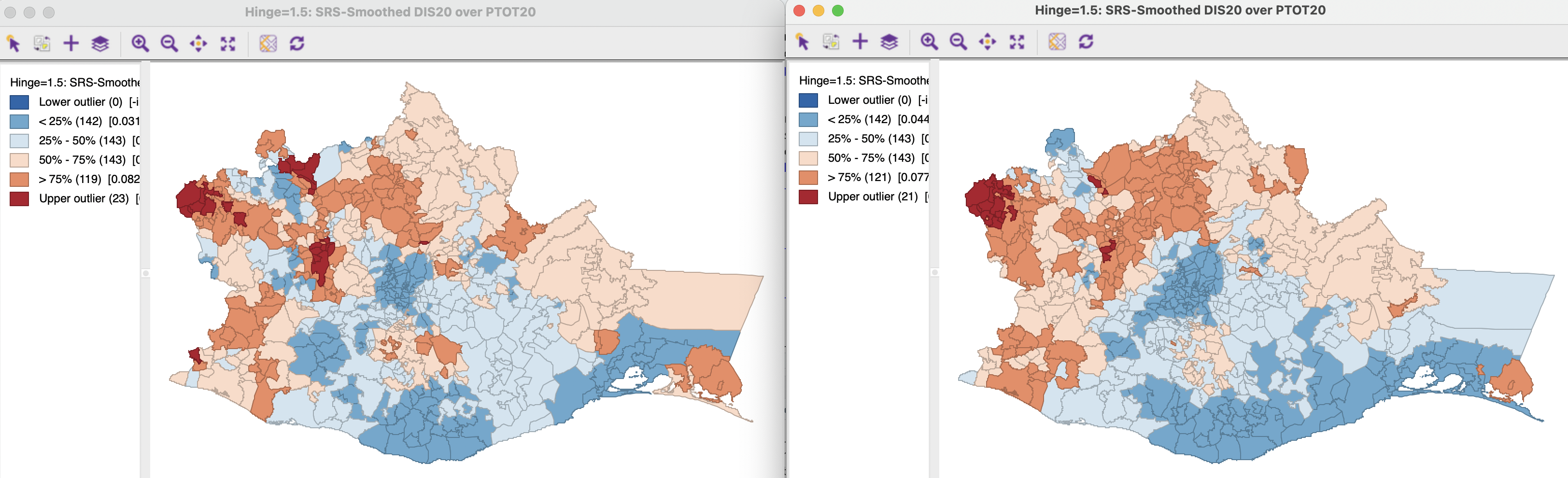
Figure 12.10: Spatial rate map: first and second order queen contiguity
Compared to the maps in Figure 12.9, a lot of detail is lost, and the emphasis is on broader regional patterns, which tend to be dominated by the data for the larger municipalities. Increasing the range of the contiguity to second order yields somewhat larger regions of similar values (in the sense of falling in the same quartile).
The spatial rate smoothing yields an even greater reduction in the variable range than the non-spatial EB. For first order contiguity, the range becomes 0.0390 to 0.1370, and for second order contiguity 0.0468 to 0.1164. In contrast to EB rates, which remain highly correlated with the original raw rate, this is no longer the case for spatially smoothed rates. The averaging over spatial units breaks the connection with the original values somewhat. In the current example, the correlation between raw rate and the two spatial rates is, respectively, 0.504 for first order and 0.468 for second order contiguity. This should be kept in mind when interpreting the results.
The spatially smoothed rate map retains all the standard options of a map in GeoDa, as well as the special options of other rate maps (see Section 6.2.2). The default variable name for the Save Rates option is R_SPAT_RT. Currently, there are no metadata that keep track of the spatial weights used in the smoothing operation.
12.4.1.2 Spatially smoothed rate in table
As is the case for other rate calculations (see, e.g., Section 6.2.2.1), the rates can also be computed by means of Table > Calculator. The only difference is that now there is also a drop down list to specify the spatial weights. All other operations are identical to the non-spatial case.
As mentioned, sometimes the use of inverse distance or kernel weights is advocated to lessen the effect of neighboring values on the computed spatial smoothed rate. While it may be tempting to carry out the rate calculation using such spatial weights, this does not work correctly in GeoDa. Figure 12.11 illustrates this issue. It portrays spatially smoothed rates using two different spatial weights. The map on the left is based on k-nearest neighbor weights, with k=6, oaxaca_k6,95 the map on the right on inverse distance weights using the 6 nearest neighbors as a variable bandwidth, oaxaca_idk6. The maps are identical because only the contiguity information is used in the weights operations.
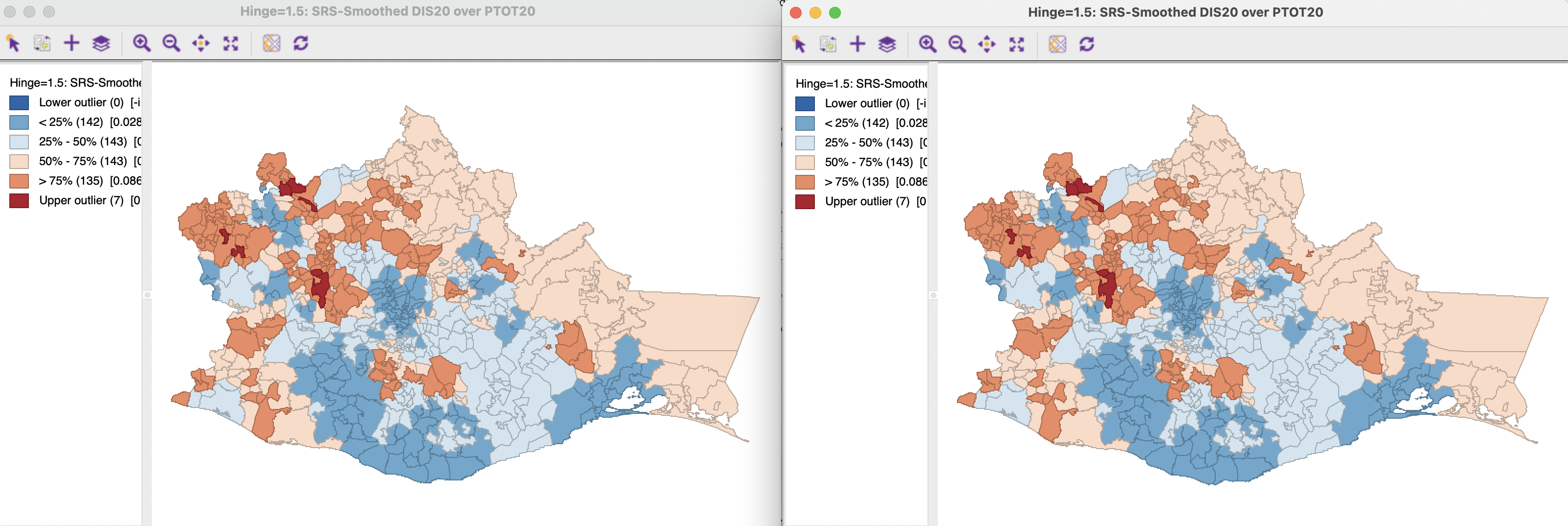
Figure 12.11: Spatial rate map: k-nearest neighbor and inverse distance weights
The proper way to compute spatially smoothed rates for inverse distance or kernel weights is through the Calculator. A spatially lagged variables must be computed separately for the numerator and denominator, using either inverse distance or kernel weights. These new variables are then used to compute a ratio, as a division operation in the calculator. Figure 12.12 shows a box map with the result (the computed variable is ID_RATE). The pattern clearly differs from that in the maps in Figure 12.11. The effect of large neighbors is lessened because of the distance decay effect embedded in the inverse distance weights.
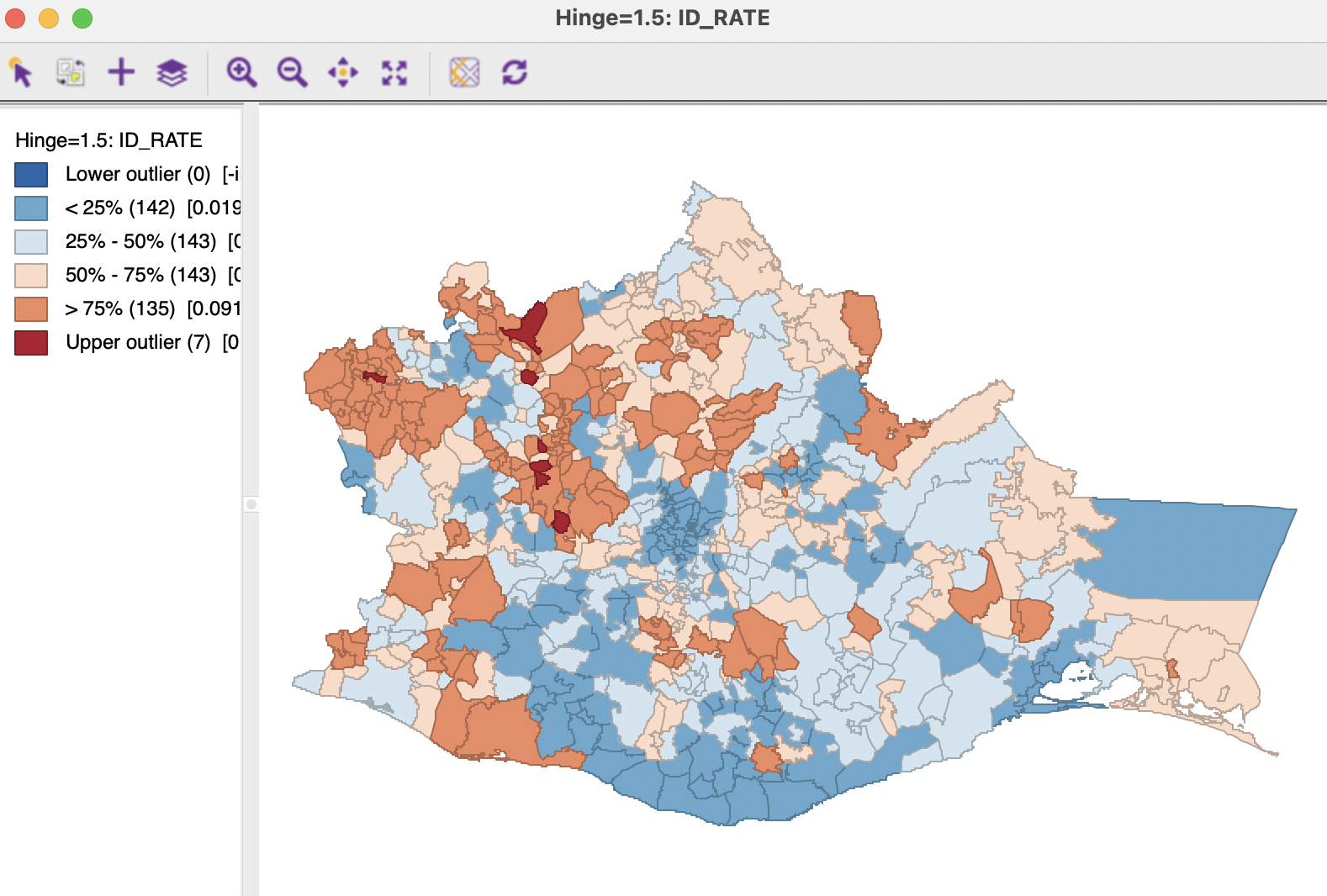
Figure 12.12: Spatial rate map: inverse distance weights from Calculator
12.4.2 Spatial Empirical Bayes Smoothing
The spatial Empirical Bayes rate smoothing method is based on the same principle as the standard Empirical Bayes smoother, covered in Chapter 6. The main difference is that the reference rate is computed for a spatial window, specific to each individual observation, rather than taking the same overall reference rate for all observations. This approach only works when the number of observations in the reference window, as defined by the spatial weights, is large enough to allow for effective smoothing. This is a context where block weights become very useful (Section 11.5.3), since they avoid the irregularity in the number of neighbors on which the reference rate is based. All the observations in the same block have an identical number of reference points from which the reference rate is computed.96
Similar to the standard EB principle, a reference rate (or prior) is computed from the data. It is estimated from the spatial window surrounding a given observation.
Formally, the reference mean for location \(i\) is then: \[\mu_i = \frac{\sum_j w_{ij} O_j}{\sum_j w_{ij} P_j},\]
with \(w_{ij}\) as binary spatial weights, and \(w_{ii} = 1\).
The local estimate of the prior variance follows the same logic as for EB, but replacing the population and rates by their local counterparts: \[\sigma^2_i = \frac{\sum_j w_{ij}[ P_j (r_i - \mu_i)^2] }{\sum_j w_{ij} P_j} - \frac{\mu_i}{\sum_j w_{ij} P_i / (k_i +1)}.\] Note that the average population in the second term pertains to all locations within the window, therefore, this is divided by \(k_i + 1\) (with \(k_i\) as the number of neighbors of \(i\)). As in the case of the standard EB rate, it is quite possible (and quite common) to obtain a negative estimate for the local variance, in which case it is set to zero.
The spatial EB smoothed rate is computed as a weighted average of the crude rate and the prior, in the same manner as for the standard EB rate (Section 6.4.2.2).
12.4.2.1 Spatial Empirical Bayes smoothed rate map
A spatial Empirical Bayes smoothed rate map is selected from the list of map options as Rates > Spatial Empirical Bayes. Alternatively, from the menu, it is obtained from Map > Rates-Calculated Map > Spatial Empirical Bayes. The map is created in exactly the same way as for the spatial rate map.
In the example, shown in Figure 12.13, block weights based on the region to which a municipality belongs (oaxaca_reg) are used to define the reference window for each observation. These weights have on average 95 neighbors, ranging from a minimum of 19 to 154. The left panel of the figure illustrates the regional division, whereas the smoothed rates are mapped in the right panel.
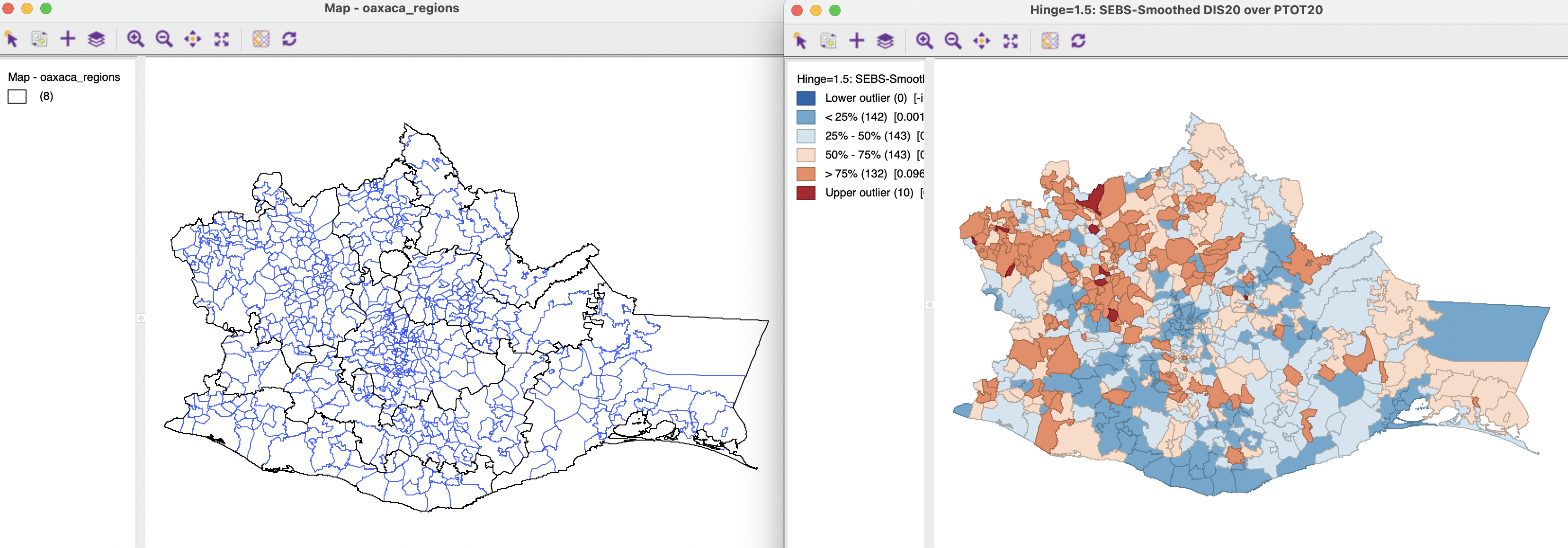
Figure 12.13: Spatial Empirical Bayes smoothed rate map using region block weights
While there are many similarities with the pattern for the standard EB rate, shown in Figure 12.9, there are also a few differences, such as an additional upper outlier and a number of observations that shift from the first quartile to the second quartile, as well as from the fourth quartile to the third. The correlation with the original EB rate is very high, at 0.996, suggesting overall a great similarity between the two results.
All the usual options are in effect. The rate can be saved with a default variable name of R_SPAT_EBS.
Since the coordinates for the Oaxaca data set are in decimal degrees latitude-longitude, the weights were constructed using Arc Distance (km) option in the Weights File Creation dialog.↩︎
Since the observation itself is included in the reference window, all observations in the same block will have the same mean and variance for the prior.↩︎