17.2 Extensions of the Local Moran
Three extensions of the Local Moran are considered. Two of these are local extensions of the specialized Moran scatter plots considered in Section 14.2.1 for the differential Moran scatter plot, and in Section 14.2.2 for the Moran scatter plot with EB rates. The third extension uses a different concept of spatial lag. Instead of the average of the values in neighboring locations, the Median Local Moran uses the median. This is considered first.
As was the case for their global counterparts, the other two extensions are primarily shortcuts to facilitate computations. They are straightforward applications of the Local Moran statistic to pre-computed variables. In one case, it is the difference between observations at two periods in time, yielding the Differential Local Moran, in the other case, rates are standardized to control for variance instability, resulting in the EB Local Moran.
17.2.1 Median Local Moran
In the discussion of spatial autocorrelation statistics so far, a spatially lagged variable was defined as \(\sum_j w_{ij} z_j\), or the average of the values observed at the neighboring locations. However, as is well known, the average may be sensitive to the presence of outliers. This may pull the average up (or down), even when many of the neighbors do not have high (low) values, creating a potentially misleading impression of a cluster or spatial outlier.
An alternative can be based loosely on the idea of a median smoother (e.g., Wall and Devine 2000). In the latter, the value at a location (typically a rate) is replaced by the median of the neighboring locations (see also Section 12.3.1.3). In the context of the Local Moran, the median of the neighbors is used in the place of the average as a median spatial lag.
Consequently, the Median Local Moran becomes: \[I_{i}^M = z_i \times \mbox{med}(z_j, j \in N_i),\] where \(N_i\) is the neighbor set of location \(i\) (i.e., those locations for which \(w_{ij} \neq 0\)).
Inference and interpretation are identical to that for the original Local Moran, based on a conditional permutation approach (see Section 16.5).
17.2.1.1 Implementation
The Median Local Moran is invoked as the second item in first group of the Cluster Maps drop down list from the toolbar, or as Space > Univariate Median Local Moran’s I from the menu.
This brings up the usual variable selection dialog. All the options are the same as for the conventional Local Moran, i.e., the randomization, significance filter and saving of the results (see Chapter 16).
These features are illustrated using the variable p_PHA(2010) (or, p_PHA10) from the Oaxaca data set, with queen contiguity. The significance map for 99,999 permutations is shown in Figure 17.1, with the result for the Median Local Moran in the right-hand panel, compared to the conventional Local Moran on the left.
Overall, with a p < 0.05 cut-off, there are 18 fewer significant locations for the Median Local Moran compared to the conventional version. These are distributed over the different categories as 10 fewer for p < 0.05, 5 fewer for p < 0.01, 2 fewer for p < 0.001, and one at p < 0.00001, but none at p < 0.0001. However, the changes work in both directions, with some locations becoming significant for the Median Local Moran, that were not for the conventional Local Moran, and the other way around. In addition, there are changes in the category of significance in both directions (both less and more significant). For example, the blue highlight in Figure 17.1 points to a municipality that was not significant for the conventional Local Moran, but becomes so at p < 0.01 for the Median Local Moran. In contrast, the red highlighted location was significant for the conventional Local Moran and becomes insignificant for the median version.
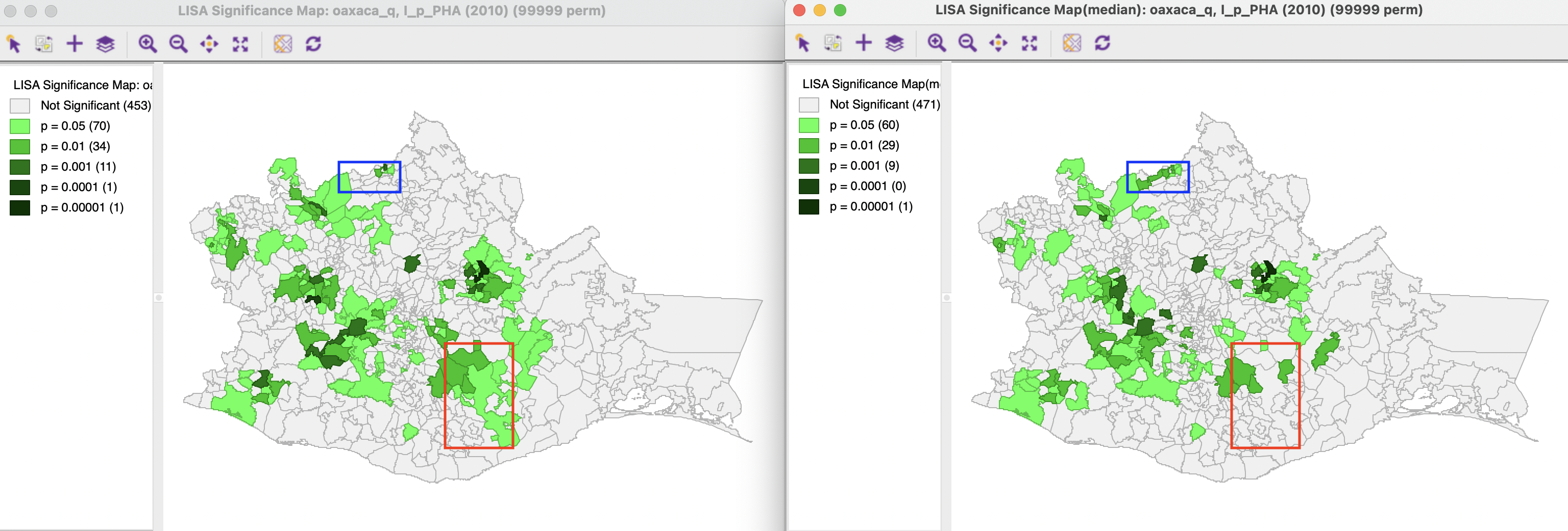
Figure 17.1: Significance maps conventional and Median Local Moran
17.2.1.2 Clusters and spatial outliers
The classification of significant locations for the Median Local Moran uses the same principle as for the conventional Local Moran, but now the reference points are the median of the (standardized) variable and the median of its median spatial lag. In a scatter plot of the median lag on the original variable, the center point is drawn at the location of the means, not the medians. Consequently, the resulting quadrants are not appropriate to derive the categories of spatial association. For example, for the standardized variable computed from p_PHA10, the mean is obviously 0 by construction, but the median is 0.1613. Similarly, the mean and median for the median spatial lag (on the vertical axis) are not the same, with the latter equal to 0.1786.
As a result, the classification into High-High or Low-Low clusters or spatial outliers must be done relative to the median values and not relative to the means shown in a conventional scatter plot.
This is further illustrated in Figures 17.2 and 17.3 for spatial clusters, and Figures 17.4 and 17.5 for spatial outliers.116
In the left-hand panel of Figure 17.2, the observations are selected that are above the median for the (standardized) variable and above the median for the median spatial lag. Clearly, this selection does not match the conventional High-High criterion based on the means. In the cluster map on the right, the subset of the selected observations that is also significant (see Figure 17.1) is classified as High-High in red, the non-significant locations are colored grey. A similar operation is carried out (under the hood) to find the Low-Low clusters, shown in Figure 17.3. In this case, since the median is above the mean for both axes, the selection includes observations that fall in different quadrants for the conventional Local Moran.
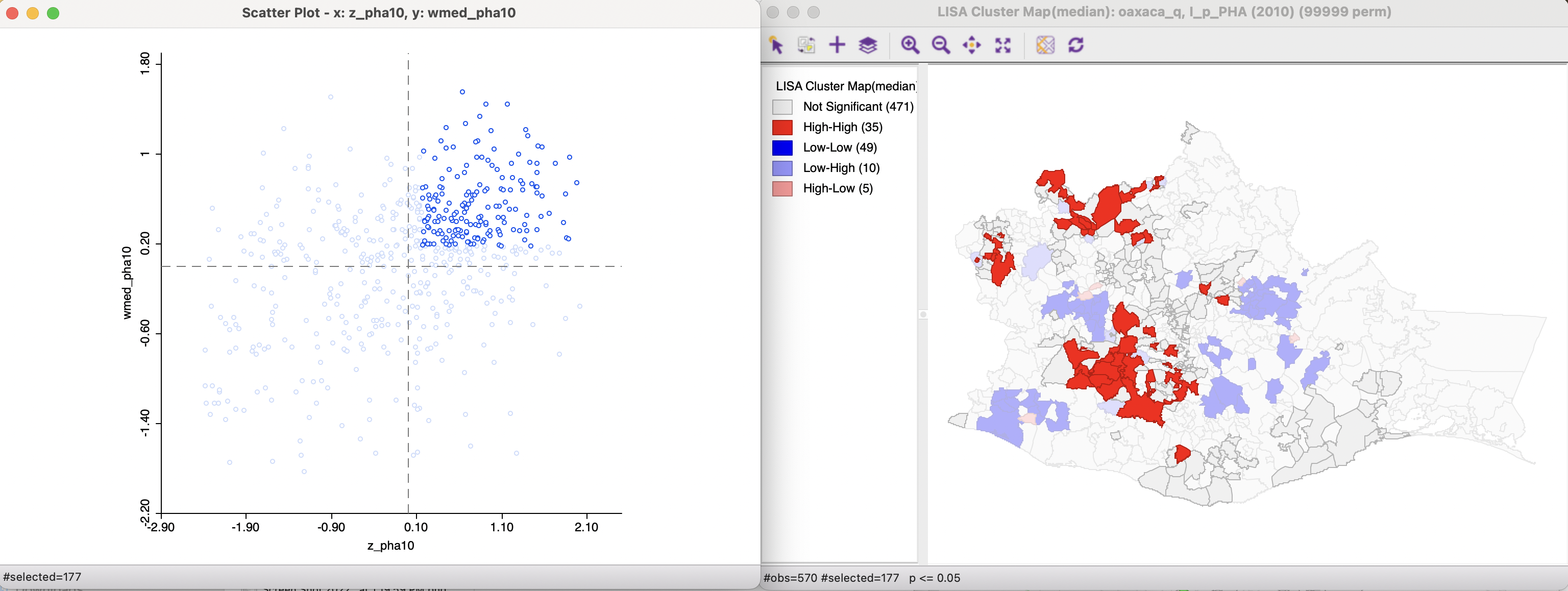
Figure 17.2: High-High clusters in Median Local Moran
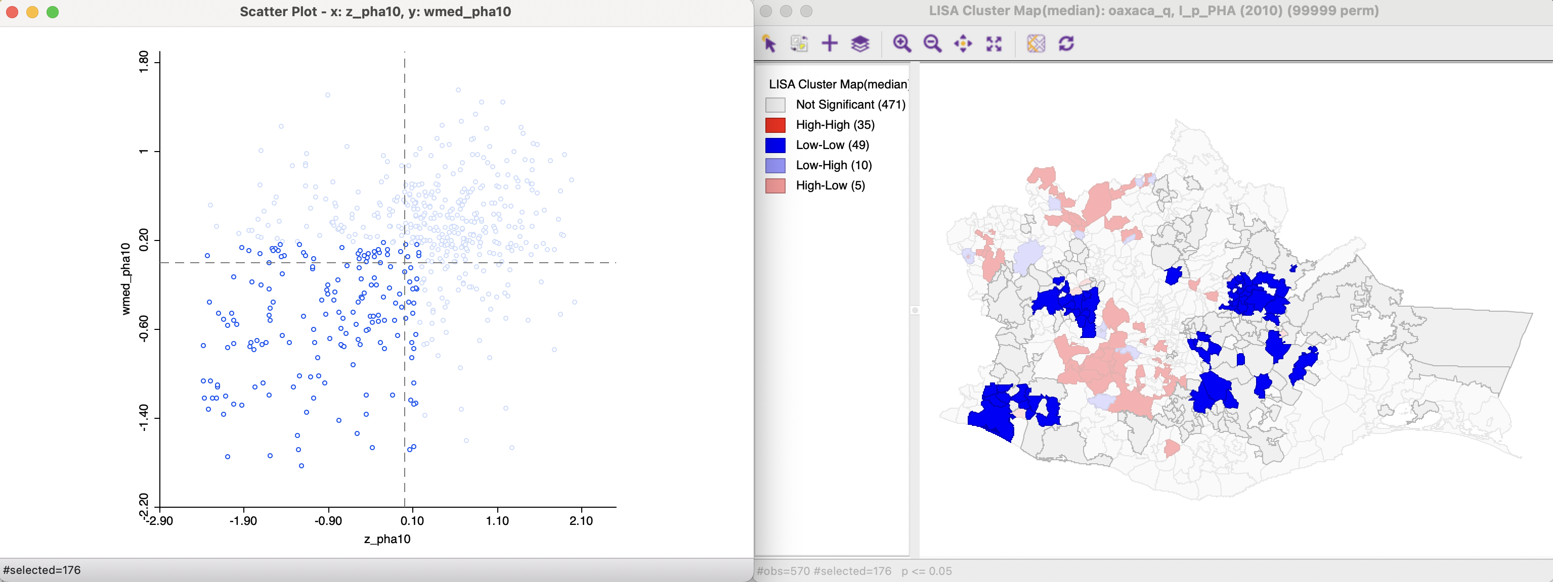
Figure 17.3: Low-Low clusters in Median Local Moran
The same principle is applied to the spatial outliers, illustrated in Figures 17.4 and 17.5. Again, the classification into the respective categories differs from what the conventional scatter plot would yield. The significant observations correspond with locations classified as spatial outliers in the cluster map on the right.
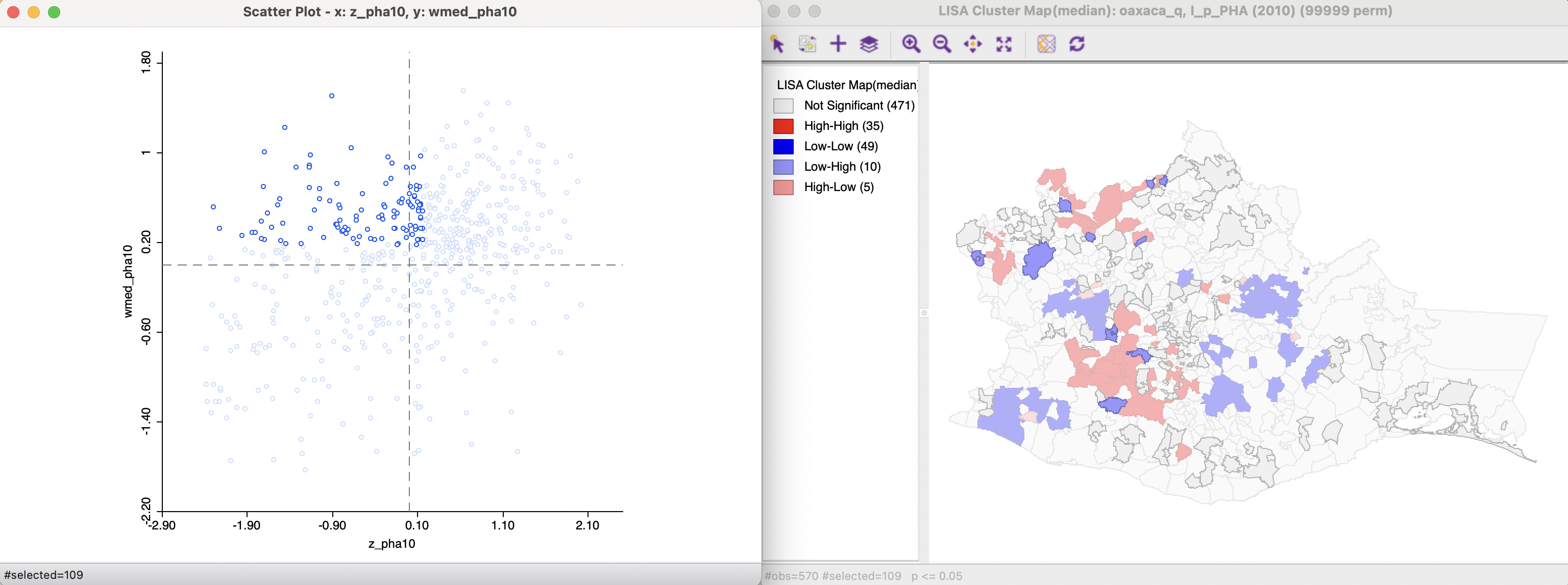
Figure 17.4: Low-High Spatial Outliers in Median Local Moran
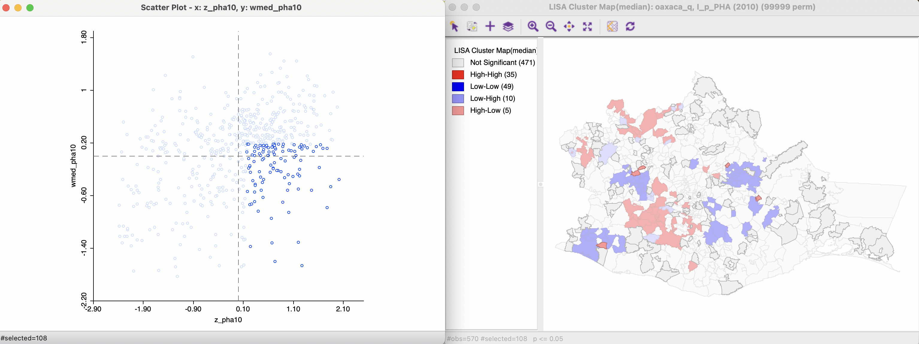
Figure 17.5: High-Low Spatial Outliers in Median Local Moran
17.2.1.3 Median Moran cluster map
A comparison of the cluster map obtained by the conventional Local Moran and the Median Local Moran (for 99,999 permutations, with p < 0.05) is illustrated in Figure 17.6. In the current example, the difference in significance results in clusters that are much more limited in range compared to the conventional Local Moran. For example, both the High-High cluster highlighted in the blue rectangle and the Low-Low cluster highlighted in the red rectangle are much smaller for the Median Local Moran. In addition, the classification of the significant locations changes as well. For example, in the green rectangle, two High-Low outliers for the conventional Local Moran become part of a Low-Low cluster.
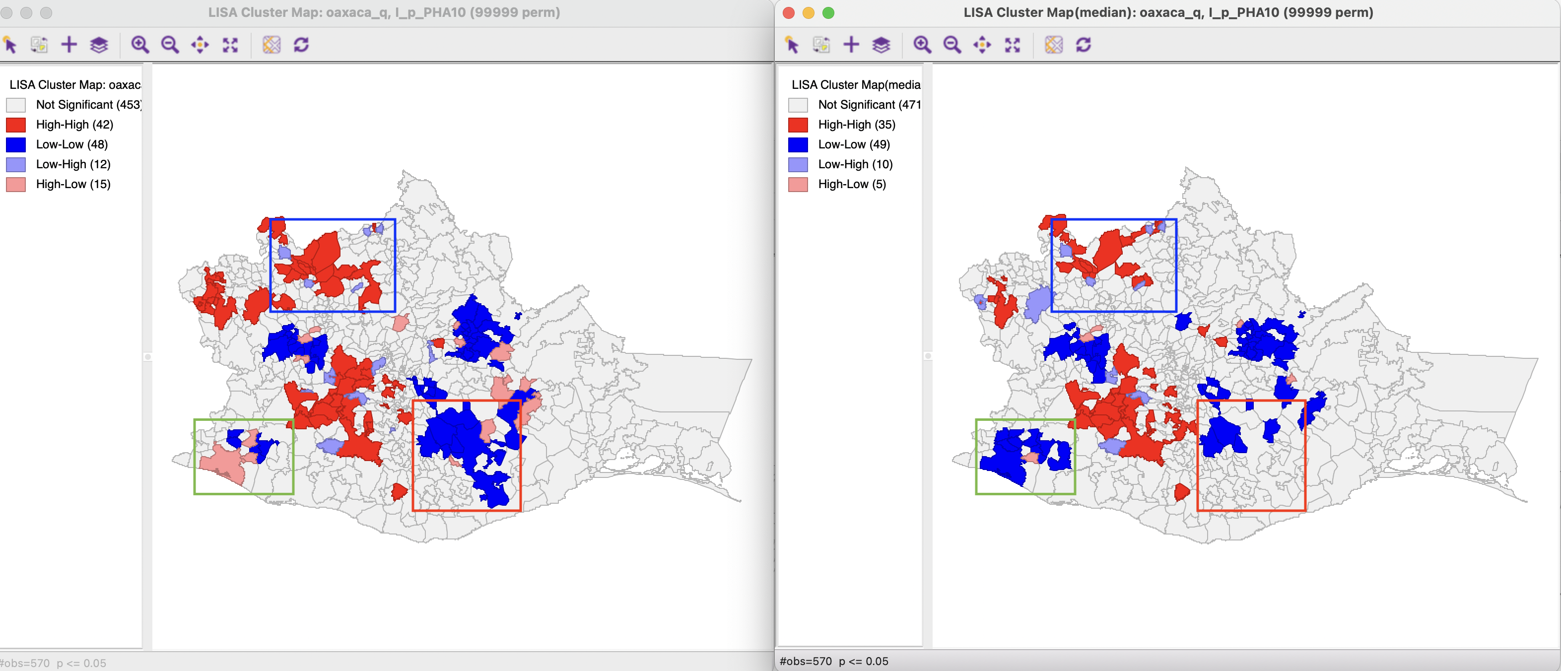
Figure 17.6: Cluster maps conventional and Median Local Moran
Overall, a comparison of the results for the Median Local Moran to the conventional Local Moran provides insight into the sensitivity of the results to potential outliers. It should be part of a standard sensitivity analysis, together with an assessment of different p-value cut-offs.
17.2.2 Differential Local Moran
The Differential Local Moran statistic is the local counterpart to the Differential Moran scatter plot, discussed in Section 14.2.1. Instead of using the observations on a variable at two different time periods separately, this statistic is based on the change over time, i.e., the difference between \(y_t\) and \(y_{t-1}\). Note that this is the actual difference and not the absolute difference, so that a positive change will be viewed as high, and a negative change as low. The differences are used in standardized form, i.e., they are not the differences between the standardized variable at two points in time, but the standardized differences between the original values for the variable.
The formal expression for this statistic follows the same logic as before, and consists of the cross product of the difference between \(y_t\) and \(y_{t-1}\) at \(i\) with the associated spatial lag:
\[I_{i}^D = a (y_{i,t} - y_{i,t-1}) \sum_j w_{ij} (y_{j,t} - y_{j,t-1}).\] The scaling constant \(a\) can be ignored. In essence, this is the same as the conventional Local Moran applied to the difference, but the implementation is based on selecting the two variables and computing the difference under the hood, rather than computing the difference separately.
As before, inference is based on conditional permutation. All the usual caveats hold about multiple comparisons and the choice of a p-value. In all respects, the interpretation is the same as for the conventional Local Moran statistic.
17.2.2.1 Implementation
The Differential Local Moran is invoked as the fourth item in first group of the Cluster Maps drop down list from the toolbar, or as Space > Differential Local Moran’s I from the menu.
As in the global case, the variables under consideration must be time-enabled (grouped) in the data table. The variable selection dialog is slightly different from the standard interface, but the same as for the differential Moran scatter plot.
Continuing to use the (time-enabled) Oaxaca data set, first, the variable of interest is selected (here, p_PHA), and then the two time periods are chosen (here, 2020 and 2010). Note that the system is agnostic about the actual time periods, so that any combination can be selected. The statistic is computed for the difference between the time period specified as the first item and that given as the second item. In the example, the spatial weights are oaxaca_q.
To provide some context, Figure 17.7 shows the cluster maps for the conventional Local Moran for p_PHA in 2010 and 2020 (using 99,999 permutations and p < 0.05). The local patterns in the two years are very different, with many High-High clusters from 2010 labeled as Low-Low in 2020, and vice versa. Note that the classification is relative to the mean, which has improved considerably between the two years (from 53.4 % to 75.8 %).
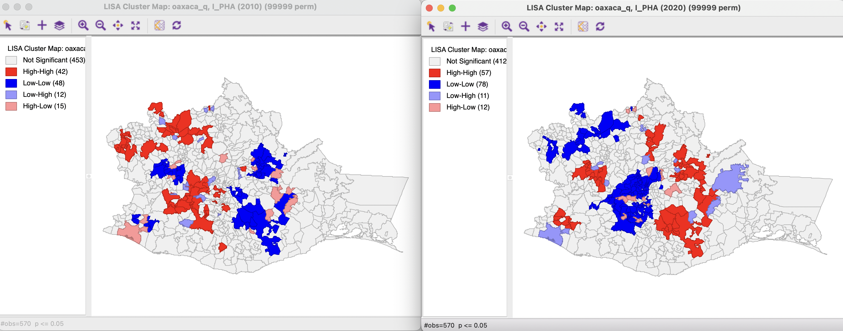
Figure 17.7: Cluster maps for Local Moran in 2010 and 2020
The significance map and cluster map for the Differential Local Moran (99,999 permutations with p < 0.05) are shown in Figure 17.8. Note how the High-High clusters correspond to locations that were Low-Low in 2010, but High-High in 2020, suggesting a grouping of large increases. Reversely, the Low-Low clusters for the difference correspond to locations that were High-High in 2010, but Low-Low in 2020, suggesting a grouping of small increases, or even decreases.
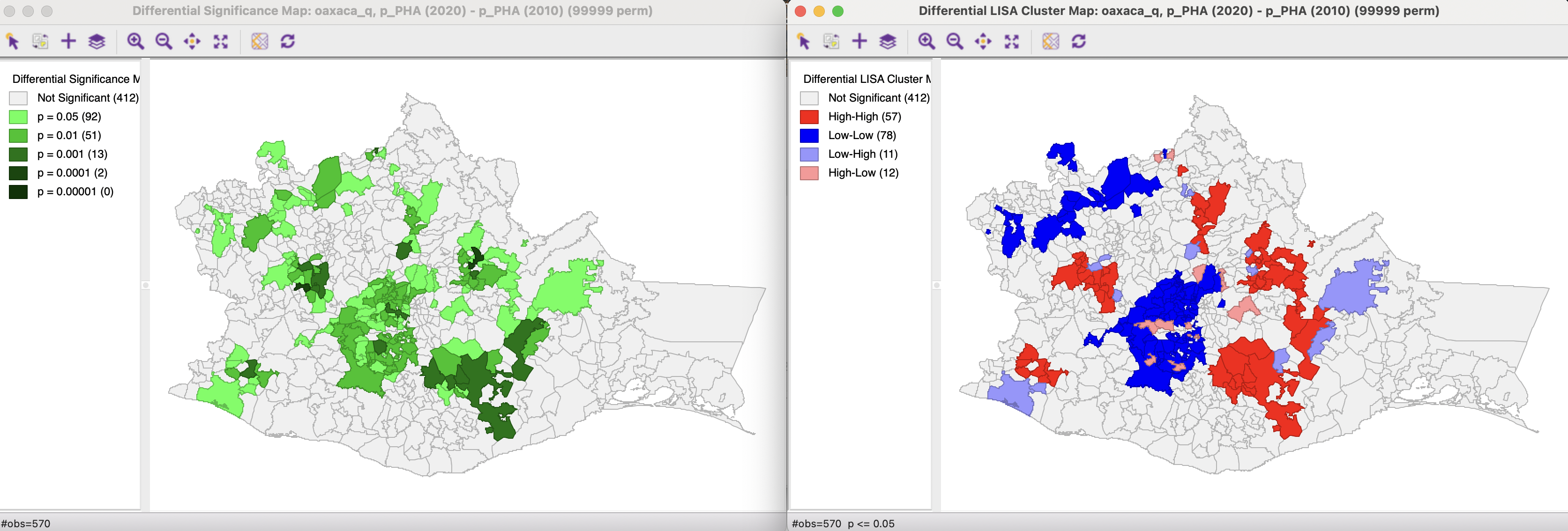
Figure 17.8: Differential Local Moran significance and cluster maps
All the options, such as randomization and significance filter are the same as for the conventional local Moran and will not be further discussed here. The only slight difference is in how the results are saved. Similar to the functionality for the differential Moran scatter plot, the Save Results option includes an item to save the actual change variable (in raw form, not in standardized form). In the dialog, this corresponds to the Diff Values item with default variable name DIFF_VAL2. The other options are the same as for all local spatial autocorrelation statistics, i.e., the value of the statistic (LISA_I), cluster type (LISA_CL), and p-value (LISA_P).
Once the difference is saved as a separate variable, it can be used in a conventional univariate Local Moran operation.
17.2.2.2 Interpretation
The significance and cluster maps for a Differential Local Moran identify the locations where the change in the variable over time is matched by similar/dissimilar changes in the surrounding locations. It is important to keep in mind that the focus is on change, and there is no direct connection to whether this changes is from high or from low values.
Two situations can be distinguished, depending on whether the change variable takes on both positive and negative values, or when all the changes are of the same sign (i.e., all observations either increase or decrease over time).
When both positive and negative change values are present, the High-High locations will tend to be locations with a large increase (positive change), surrounded by locations with similar large increases. The Low-Low locations will be observations with a large decrease (negative change), surrounded by locations with similar large decreases. Spatial outliers will be locations where an increase is surrounded by a decrease and vice versa.
When all changes are of the same sign, the interpretation of High-High and Low-Low is relative to the mean. When all the changes are positive, large increases surrounded by other large increases will be labeled High-High, whereas small(er) increases surrounding by other small(er) increases will be labeled Low-Low. When all the signs are negative, small(er) decreases surrounded by other small(er) decreases will be labeled as High-High, whereas large decreases surrounded by other large decreases will be labeled Low-Low.
17.2.3 Local Moran with EB Rate
The third extension of the Local Moran pertains to the special case where the variable of interest is a rate or proportion. As discussed for the Moran scatter plot in Section 14.2.2, the resulting variance instability can cause problems for the Moran statistic. The EB standardization suggested by Assunção and Reis (1999) for the global case can be extended to the local statistic in a straightforward manner. The statistic has the usual form, but is computed for the standardized rates, \(z\):
\[I_{i}^{EB} = a z_i \sum_j w_{ij} z_j,\] The standardization of the raw rate \(r_i\) is the same as before, and is repeated here for completeness (for a more detailed discussion, see Section 14.2.2):
\[z_i = \frac{r_i - \beta}{\sqrt{\alpha + (\beta/P_i)}}\]
with \(\beta\) as an estimate of the mean and the denominator as an estimate of the standard error.117
All inference and interpretation is the same as for the conventional case and is not further pursued here.
17.2.3.1 Implementation
The local Moran functionality for standardized rates is invoked as the last item in the Moran group on the Cluster Maps toolbar icon. Alternatively, it can be selected from the menu as Space > Local Moran’s I with EB Rate.
Since the rate standardization is computed as part of the operation, the variable selection interface is similar to that used for rate maps. To illustrate this feature, the rate is computed with DIS20 (number of people with disabilities in 2020) as the Event Variable, and PTOT20 (total population in 2020) as the Base Variable, as done earlier in Section 14.2.2.1. A box map of the raw rate is shown in the left hand panel of Figure 12.9. The spatial weights are queen contiguity, oaxaca_q.
The resulting significance map is shown in the right-hand panel of Figure 17.9, next to the corresponding map for the crude rate (for 99,999 permutations with p < 0.05). Compared to the map for the crude rate, there is one more significant location. Interestingly, the main difference is at the high end of the significance, where the EB Local Moran has slightly more significant locations. For example, the location highlighted in the blue rectangle is significant at p < 0.00001 for EB Local Moran, but at p < 0.001 for the crude rate. Similarly, the location highlighted in the red rectangle is significant at p < 0.001 for the EB Local Moran, but at p < 0.01 for the crude rate. Since the same number of permutations is used in both cases, the p-values are comparable. Overall, however, the differences are minimal and rather subtle, confirming the findings for the Moran scatter plot.
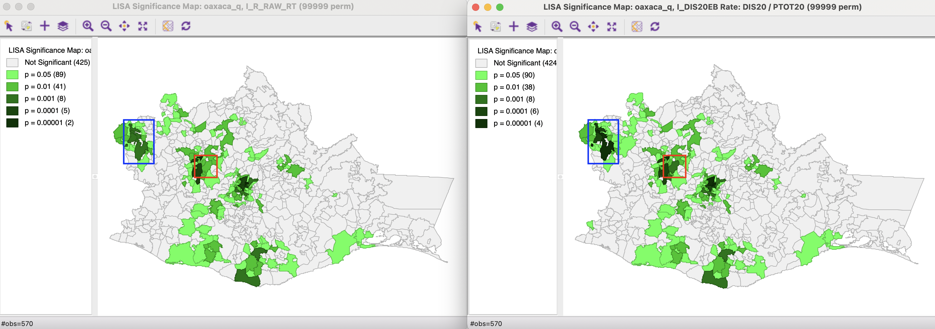
Figure 17.9: Significance maps - raw rate and EB rate
The differences between the cluster map for the crude rate and for the EB Local Moran, shown in Figure 17.10, are equally subtle. The EB Local Moran cluster map has three more locations in the High-High group, and one less in each of the Low-High and High-Low spatial outliers. Otherwise, the identified locations and groups match exactly.
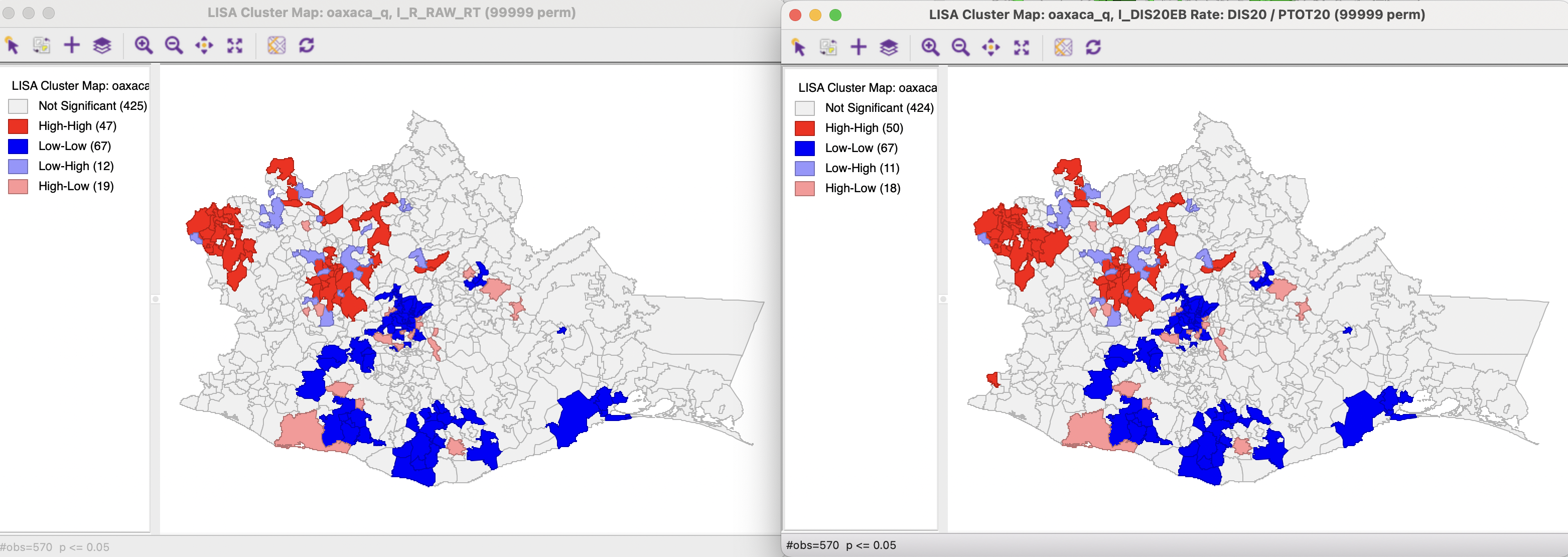
Figure 17.10: Cluster maps - raw rate and EB rate
17.2.3.2 Saving the results
As for the EB Moran scatter plot, the Save Results option includes an item to save the actual EB rate. This operation is similar to the EB Rate standardization that can be computed with the Table Calculator option (see Section 6.4.3.2). In the dialog, it corresponds to the EB Rates item, with default variable name LISA_EB. The other options are the same as for all local spatial autocorrelation statistics, i.e., the value of the statistic, cluster type, and p-value, with the same default variable names.
The selection is obtained using two steps in the Selection Tool: first selecting the observations that meet the criterion for the variable, followed by a Select From Current Selection for the median spatial lag.↩︎
To recap, \(\beta = \sum_i O_i / \sum_i P_i\), where \(O_i\) is the number of events at \(i\) and \(P_i\) is the population at risk. The estimate of \(\alpha = [\sum_i P_i ( r_i - \beta )^2 ] / P - \beta / ( P / n),\), with \(n\) as the total number of observations, such that \(P/n\) is the average population. Note that the estimate of \(\alpha\) can be negative, in which case it is set to zero.↩︎