20.5 HDBSCAN

HDBSCAN was originally proposed by Campello, Moulavi, and Sander (2013), and more recently elaborated upon by Campello et al. (2015) and McInnes and Healy (2017).¹³¹ As in DBSCAN*, the algorithm implements the notion of mutual reachability distance. However, rather than applying a fixed value of the cut-off distance to produce a cluster solution, a hierarchical process is implemented that finds an optimal cluster combination, using a different critical cut-off distance for each cluster. In order to accomplish this, the concept of cluster stability or persistence is introduced. Optimal clusters are selected based on their relative excess of mass value, which is a measure of their persistence.

HDBSCAN keeps the notion of Min Points from DBSCAN, and also uses the concept of core distance of an object (\(d_{core}\)) from DBSCAN*. The core distance is the distance between an object and its k-nearest neighbor, where k = Min Points - 1 (in other words, as for DBSCAN, the object itself is included in Min Points).

Intuitively, for the same k, the core distance will be much smaller for densely distributed points than for sparse distributions. Associated with the core distance for each object \(x\) is the concept of density or \(\lambda_p\), as the inverse of the core distance. As the core distance becomes smaller, \(\lambda\) increases, indicating a higher density of points.

As in DBSCAN*, the mutual reachability distance is employed to construct a minimum spanning tree, or, rather, the associated dendrogram from single linkage clustering. From this, HDBSCAN derives an optimal solution, based on the notion of persistence or stability of the cluster.

20.5.1 Important Concepts

Several new concepts are introduced in the treatment of HDBSCAN.

20.5.1.1 Level Set

A first general concept is that of a level set associated with a given density level \(\lambda\). This is introduced in the context of bump hunting, or the search for high density regions in a general distribution \(f\). Formally, the level set associated with density \(\lambda\) in the associated distribution is: \[L(\lambda; f) = \{ x | Prob(x) > \lambda\},\] i.e., the collection of data points \(x\) for which the probability density exceeds the given threshold. A subset of such points that contains the maximum number of points that are connected (so-called connected components) is called a density-contour cluster of the density function. A density-contour tree is then a tree formed of nested clusters that are obtained by varying the level \(\lambda\) (Hartigan 1975; Müller and Sawitzki 1991; Stuetzle and Nugent 2010).

To visualize this concept, the data distribution can be represented as a two-dimensional profile, as in Figure 20.13 (loosely based on the example in Stuetzle and Nugent 2010). A level set consists of those data points (i.e., areas under the curve) that are above a horizontal line at \(p\). This can be thought of as islands sticking out above the ocean, where the ocean level corresponds with \(p\).

For the lowest p-values in the figure, up to around 0.03, all the land mass is connected and it appears as a single entity. As the p-value increases, part of the area gets submerged and two separate islands appear, with a combined land mass (level set) that is smaller than before. Each of these land masses constitutes a density-contour cluster. As the p-value becomes larger than around 0.08, the island to the right disappears, and only a single island remains, corresponding to a yet smaller level set. Finally, for p > 0.10, this splits into two separate islands.

The level set establishes the connection between the density and the cluster size.

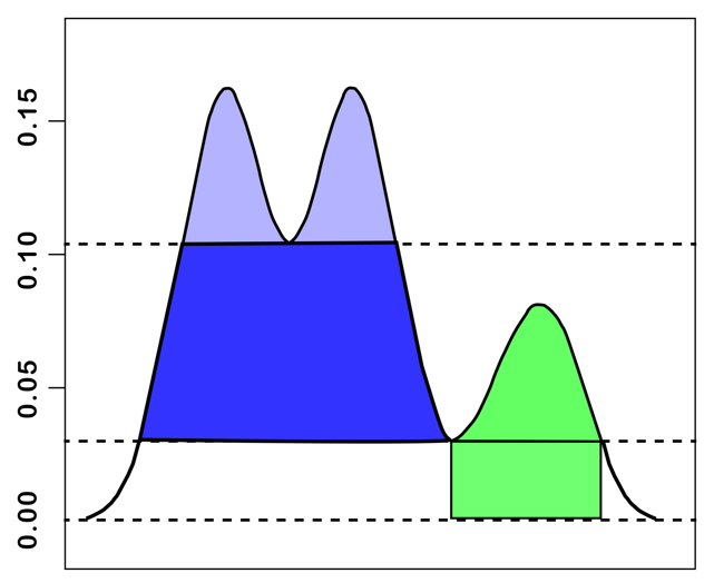
Figure 20.13: Level Set

20.5.1.2 Persistence and Excess of Mass

As the value of the density \(\lambda\) increases, or, equivalently, as the core distance becomes smaller, larger clusters break into sub-clusters (the analogy with rising ocean levels), or shed Noise points. In the current context and in contrast to the previous discussion, a Noise point dropping out is not considered a split of the cluster. The cluster remains, but only becomes smaller.

The objective is to identify the most prominent clusters as those that continue to exist longest. In the Figure, it corresponds with the area under the curve while a particular cluster configuration exists. This is formalized through the concept of excess of mass (Müller and Sawitzki 1991), or the total density contained in a cluster after it is formed. The point of formation is associated with a minimum density, or \(\lambda_{min}\).

In the island analogy, \(\lambda_{min}\) would correspond to the ocean level where the land bridge is first covered by water, such that the islands appear for the first time as separate entities. The excess of mass would be the volume of the island above that ocean level, as illustrated in Figure 20.13.

The stability or persistence of a cluster is formalized through a notion of relative excess of mass of the cluster. For each cluster \(C_i\), there is a minimum density, \(\lambda_{min} (C_i)\), where it comes into being. In addition, for each point \(x_j\) that belongs to the cluster, there is a maximum density \(\lambda_{max}(x_j,C_i)\) after which it no longer belongs to the cluster. For example, in Figure 20.13, the cluster on the left side comes into being at p = 0.03. At p = 0.10, it splits into two new clusters. So, for the large cluster, \(\lambda_{min}\), or the point where the cluster comes into being is 0.03. The cluster stops existing (it splits) for \(\lambda_{max}\) = 0.10. In turn, p = 0.10 represents \(\lambda_{min}\) for the two smaller clusters. In this example, all the members of the cluster exit at the same time, but in general, this will not be the case. Individual points that fail to meet the critical distance as it decreases (\(\lambda\) increases) will fall out. Such points will therefore have a different \(\lambda_{max}(x_j,C_i)\) from those that remain in the cluster. They are treated as Noise points, while the cluster itself continues to exist.

The persistence of a given cluster \(C_i\) is then the sum of the difference between the \(\lambda_{max}\) and \(\lambda_{min}\) for each point \(x_j\) that belongs to the cluster at its point of creation: \[S(C_i) = \sum_{x_j \in C_i} [\lambda_{max}(x_j,C_i) - \lambda_{min} (C_i)],\] where \(\lambda_{min} (C_i)\) is the minimum density level at which \(C_i\) exists, and \(\lambda_{max}(x_j,C_i)\) is the density level after which point \(x_j\) no longer belongs to the cluster.

The persistence of a cluster becomes the basis to decide whether to accept a cluster split or to keep the larger entity as the cluster.

20.5.1.3 Condensed dendrogram

A condensed dendrogram is obtained by evaluating the stability of each cluster relative to the clusters into which it splits. If the sum of the stability of the two descendants (or children) is larger than the stability of the parent node, then the two children are kept as clusters and the parent is discarded. Alternatively, if the stability of the parent is larger than that of the children, the children and all their descendants are discarded. In other words, the large cluster is kept and all the smaller clusters that descend from it are eliminated. Here again, a split that sheds a single point is not considered a cluster split, but only a shrinking of the original cluster (which retains its label). Only true splits that result in sub-clusters that contain at least two observations are considered in the simplification of the tree.

Sometimes a further constraint is imposed on the minimum size of a cluster, which would pertain to the splits as well. As suggested in Campello et al. (2015), a simple solution is to set the minimum cluster size equal to Min Points.

For example, in the illustration in Figure 20.13, the area in the left cluster between 0.03 and 0.10 (in blue) is larger than the sum of the areas in the smaller clusters obtained at 0.10 (in purple). As a result, the latter would not be considered as separate clusters. The condensed dendrogram yields a much simpler tree representation and an identification of clusters that maximize the sum of the individual cluster stabilities.

20.5.2 HDBSCAN Algorithm

The HDBSCAN algorithm has the same point of departure as DBSCAN*, i.e., a minimum spanning tree or dendrogram derived from the mutual reachability distance. To illustrate the logic, the same toy example is employed as in Figure 20.5. To keep matters simple, the Min Cluster Size and Min Points are set to 2. As a result, the mutual reachability distance is the same as the nearest neighbor distance. Since the core distance for each point is its smallest distance to have one neighbor, the maximum of the two core distances and the actual distance will always be the actual distance. While this avoids one of the innovations of the algorithm, it still allows to highlight its distinctive features.

The nearest neighbor distances can be taken from the connectivity graph in Figure 20.5, which yields the core distance for each point. The \(\lambda_p\) value associated with this core distance is its inverse. The results for each point in the example are summarized in Figure 20.14.

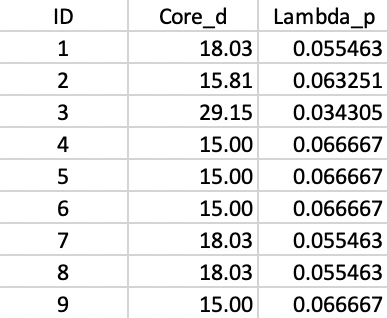
Figure 20.14: Core distance and lambda for each point

The inter-point distances form the basis for a minimum spanning tree (MST), which is essential for the hierarchical nature of the algorithm. The corresponding connectivity graph is shown in Figure 20.15, with both the node identifiers and the edge weights listed (the distance between the two nodes the edge connects). The HDBSCAN algorithm essentially consists of a succession of cuts in the connectivity graph. These cuts start with the highest edge weight and move through all the edges in decreasing order of the weight. The process of selecting cuts continues until all the points are singletons and constitute their own cluster. Formally, this is equivalent to carrying out single linkage hierarchical clustering based on the mutual reachability distance matrix.

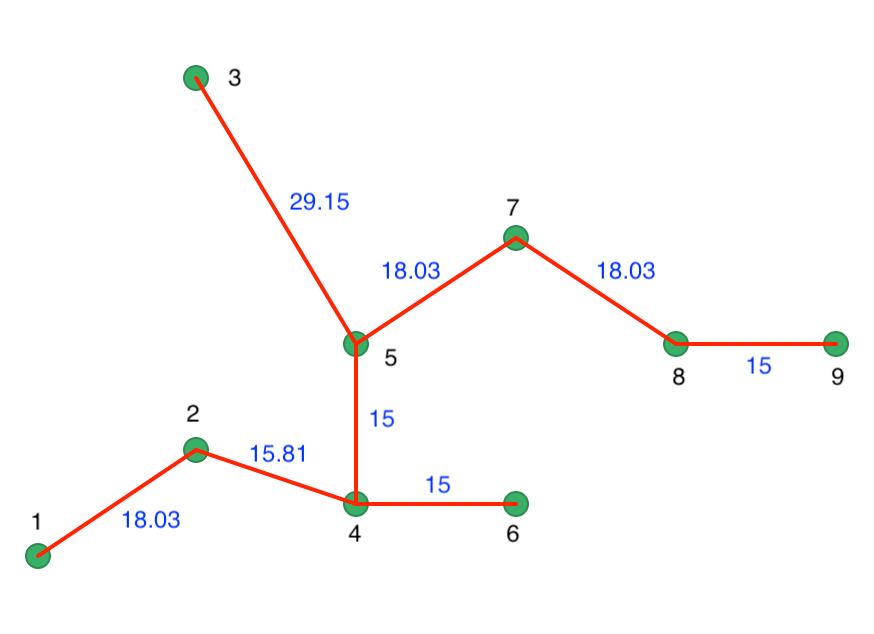
Figure 20.15: Minimum Spanning Tree Connectivity Graph

20.5.2.1 Minimum spanning tree

An alternative visualization of the pruning process is in the form of a tree, shown in Figure 20.16. In the root node, all the points form a single cluster. The corresponding \(\lambda\) level is set to zero. As \(\lambda\) increases, or, equivalently, the core distance decreases, points fall out of the cluster, or the cluster splits into two sub-clusters. This process continues until each point is a leaf in the tree (i.e., it is by itself).

In Figure 20.15, the longest edge is between 3 and 5, with a core distance of 29.15 for point 3. The corresponding \(\lambda\) is 0.034, for which point 3 is removed from the tree and becomes a leaf. In the GeoDa implementation of HDBSCAN, singletons are not considered to be valid clusters, so node C1 becomes the new root, with \(\lambda_{min}\) reset to zero.

The next meaningful cut is for \(\lambda = 0.055\), or a distance of 18.03. This creates two clusters, one consisting of the six points 1-7, but without 3, labeled C2, and the other consisting of 8 and 9, labeled C3. The process continues for increasing values of \(\lambda\), although in each case the split involves a singleton and no further valid clusters are obtained. This leads to the consideration of the stability of the clusters and the condensed tree.

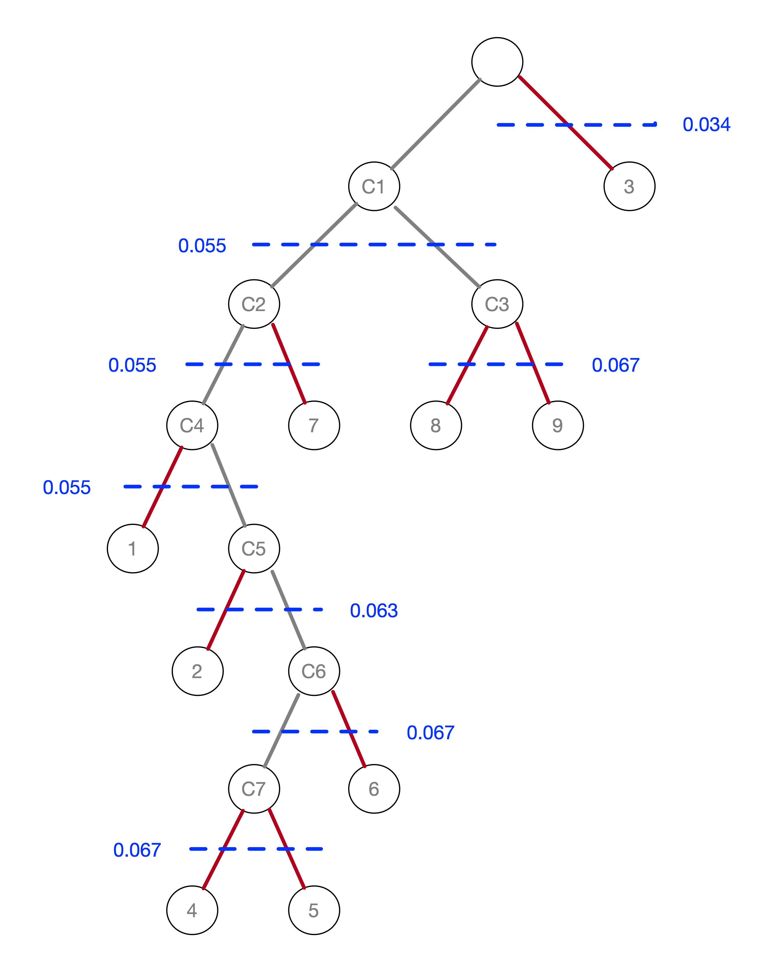
Figure 20.16: Pruning the MST

20.5.2.2 Cluster stability and condensed tree

A closer investigation of the cuts in the tree reveals that the \(\lambda_p\) values associated with each point (Figure 20.14) correspond to the \(\lambda\) value where the corresponding point falls out of a clusters in the tree. For example, for point 7, this happens for \(\lambda\) = 0.055, or a core distance of 18.03.

The stability or persistence of each cluster is defined as the sum over all the points of the difference between \(\lambda_p\) and \(\lambda_{min}\), where \(\lambda_{min}\) is the \(\lambda\) level where the cluster forms.

For example, cluster C3 is formed (i.e., splits off from C1) for \(\lambda\) = 0.055463 and consists of points 8 and 9. Therefore, the value of \(\lambda_{min}\) for C3 is 0.055463. The value of \(\lambda_p\) for points 8 and 9 is 0.066667, corresponding with a distance of 15.0 at which they become singletons (or leaves in the tree). The contribution of each point to the persistence of the cluster C3 is thus 0.066667 - 0.055463 = 0.011204. The total value of the persistence of cluster C3 is therefore the sum of this contribution for both points, or 0.022408. Similar calculations yield the persistence of cluster C2 as 0.041400. This is summarized in Figure 20.17. For the sake of completeness, the results for cluster C1 are included as well, although those are ignored by the algorithm, since C1 is reset as root of the tree.

The condensed tree only includes C1 (as root), C2 and C3. For example, the split of C2 into C4 and 7 is based on the following rationale. Since the persistence of a singleton is zero, and C4 includes one less point than C2, but with the same value for \(\lambda_{min}\), the sum of the persistence of C4 and 7 is less than the value for C2, hence the condensed tree stops there.

The condensed tree allows for different values of \(\lambda\) to play a role in the clustering mechanism, potentially corresponding with a separate critical cut-off distance for each cluster.

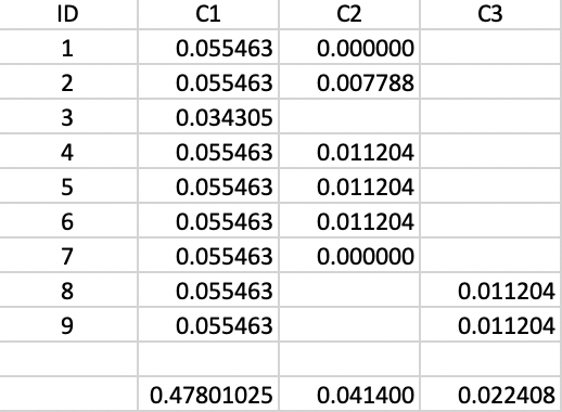
Figure 20.17: Cluster Stability

20.5.3 Cluster Membership

As outlined in the previous section, a point becomes part of a cluster for \(\lambda_{min}\), which corresponds of a cut-off distance \(d_{max}\). Once a point is part of a cluster, it remains there until the threshold distance is small enough such that it becomes Noise, which happens for \(d_{p,core}\). This may be the same or be different from the smallest distance where the cluster still exists, or \(d_{min}\). The strength of the cluster membership of point \(p\) can now be expressed as the ratio of the final cut-off distance to the core distance for point p, \(d_{max} / d_{p,core}\), or, equivalently, as the ratio of the density that corresponds to the point’s core distance to the maximum density, or, \(\lambda_{p} / \lambda_{max}\).

The ratio gives a measure of the degree to which a point belongs to a cluster. For example, for points that meet the \(d_{min}\) thresholds, i.e., observations in the highest density region, the ratio will be 1. Noise points are assigned 0. More interestingly, for points that are part of the cluster when it forms, but drop out during the pruning process, the ratio will have a value smaller than 1. Therefore, the higher the ratio, the stronger the membership of the point in the corresponding cluster.

This ratio can be exploited as the basis of a soft or fuzzy clustering approach, in which the degree of membership in a cluster is considered. This is beyond the current scope. Nevertheless, the ratio, or probability of cluster membership, remains a useful indicator of the extent to which the cluster is concentrated in high density points.

20.5.4 Outliers

Related to the identification of density clusters is a concern to find points that do not belong to a cluster and are therefore classified as outliers. Parametric approaches are typically based on some function of the spread of the underlying distribution, such as the well-known 3-sigma rule for a normal density.¹³²

An alternative approach is based on non-parametric principles. Specifically, the distance of an observation to the nearest cluster can be considered as a criterion to classify outliers. Campello et al. (2015) proposed a post-processing of the HDBSCAN results to characterize the degree to which an observation can be considered an outlier. The method is referred to as GLOSH, which stands for Global-Local Outlier Scores from Hierarchies.

The logic underlying the outlier detection is closely related to the notion of cluster membership just discussed. In fact, the probability of being an outlier is the complement of the cluster membership.

The rationale behind the index is to compare the density threshold for which the point is still attached to a cluster (\(\lambda_p\) in the previous discussion) and the highest density threshold \(\lambda_{max}\) for that cluster. The GLOSH index for a point \(p\) is then: \[\mbox{GLOSH}_p = \frac{\lambda_{max} - \lambda_p}{\lambda_{max}},\] or, equivalently, \(1 - \lambda_p / \lambda_{max}\), the complement of the cluster membership for all but Noise points. For the latter, since the cluster membership was set to zero, the actual \(\lambda_{min}\) needs to be used. Given the inverse relationship between density and distance threshold, an alternative formulation of the outlier index is as: \[\mbox{GLOSH}_p = 1 - \frac{d_{min}}{d_{p,core}}.\]

20.5.5 Implementation

HDBSCAN is invoked from the Menu or the cluster toolbar icon (Figure 20.7) as the second item in the density clusters subgroup, Clusters > HDBSCAN. The overall setup is very similar to that for DBSCAN, except that there is no threshold distance. Again, the coordinates are taken as XKM and YKM.

The two main parameters are Min Cluster Size and Min Points. These are typically set to the same value, but there may be instances where a larger value for Min Cluster Size is desired. In the illustration, these values are set to 10. The Min Points parameter drives the computation of the core distance for each point, which forms the basis for the construction of the minimum spanning tree. As before, Transformation is set to Raw and Distance Function to Euclidean.

The Run button brings up a cluster map and the associated dendrogram. The cluster map, shown in Figure 20.18, reveals 7 clusters, ranging in size from 67 to 10, with 69 Noise points. The Summary button reveals an overall fit of 0.970, which is the best value achieved so far.

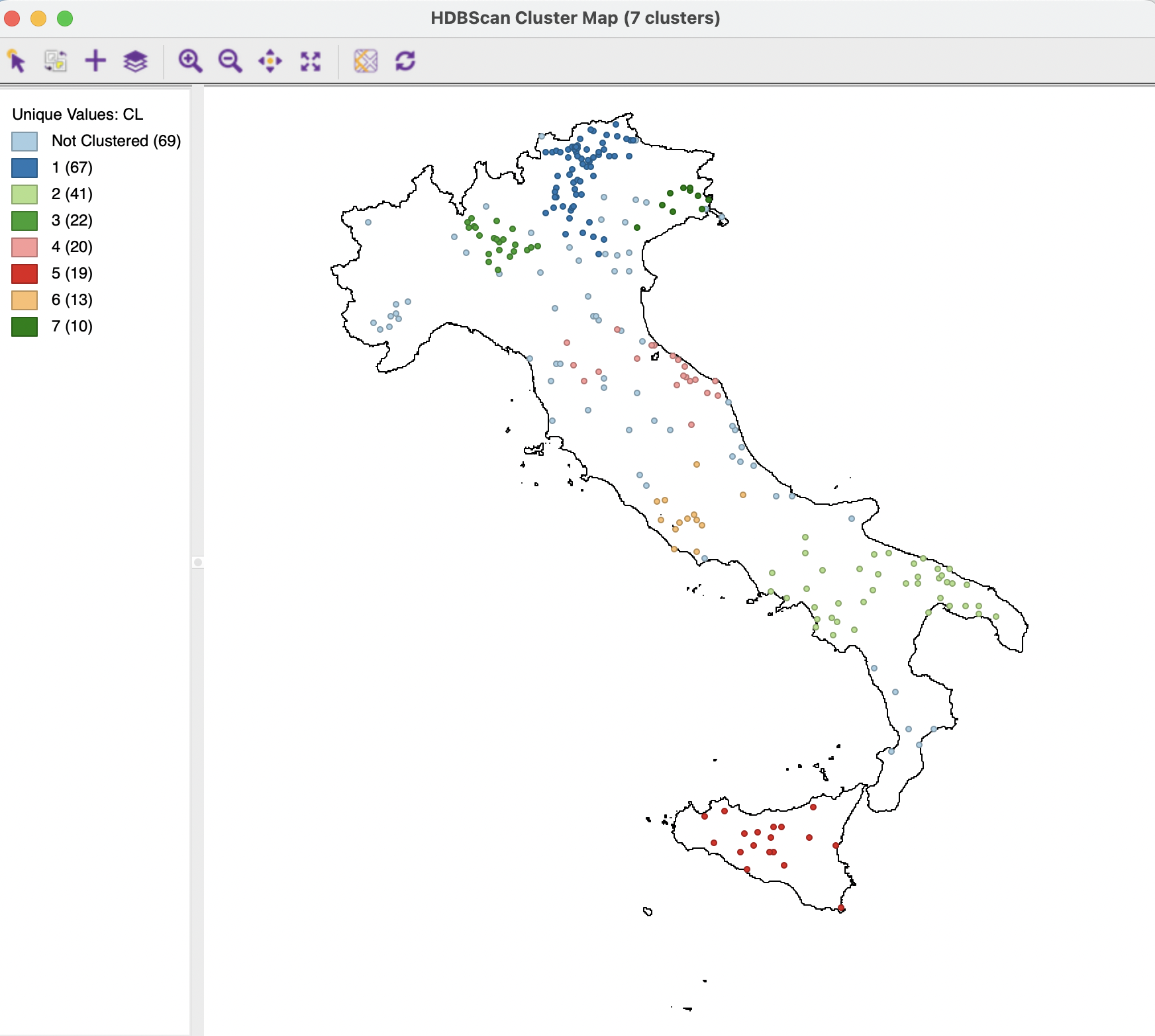
Figure 20.18: HDBSCAN Cluster Map

In and of itself, the raw dendrogram is not of that much interest. One interesting feature of the dendrogram in GeoDa is that it supports linking and brushing, which makes it possible to explore what branches in the tree subsets of points or clusters belong to (selected in one of the maps). The reverse is supported as well, so that branches in the tree can be selected and their counterparts identified in other maps and graphs.

In Figure 20.19, the 19 observations are selected that form cluster 5, consisting of bank locations on the island of Sicily. The corresponding branches in the dendrogram are highlighted. This includes all the splits that are possible after the formation of the final cluster, in contrast to the condensed tree, considered next.

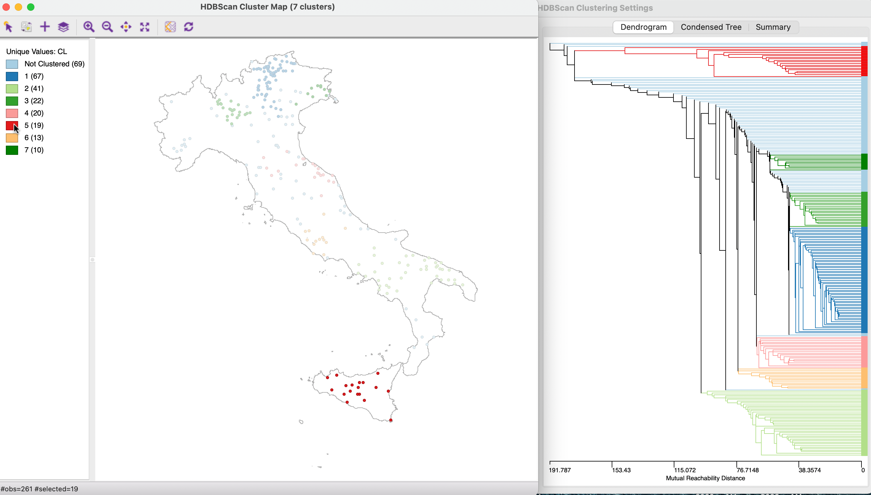
Figure 20.19: HDBSCAN Dendrogram

20.5.5.1 Exploring the condensed tree

An important and distinct feature of the HDBSCAN method is the visualization of cluster persistence (or stability) in the condensed tree or condensed dendrogram. This is invoked by means of the middle button in the results panel. The tree visualizes the relative excess of mass that results in the identification of clusters for different values of \(\lambda\). Starting at the root (top), with \(\lambda\) = 0, the left hand axis shows how increasing values of \(\lambda\) (going down) results in branching of the tree. The shaded areas are not rectangles, but they gradually taper off, as single points are shredded from the main cluster.

The optimal clusters are identified by an oval with the same color as the cluster label in the cluster map. The shading of the tree branches corresponds to the number of points contained in the branch, with lighter suggesting more points. In Figure 20.20, the same 19 members of cluster 5 are selected as before. In contrast to the dendrogram, no splits occur below the formation of the cluster, highlighted in red.

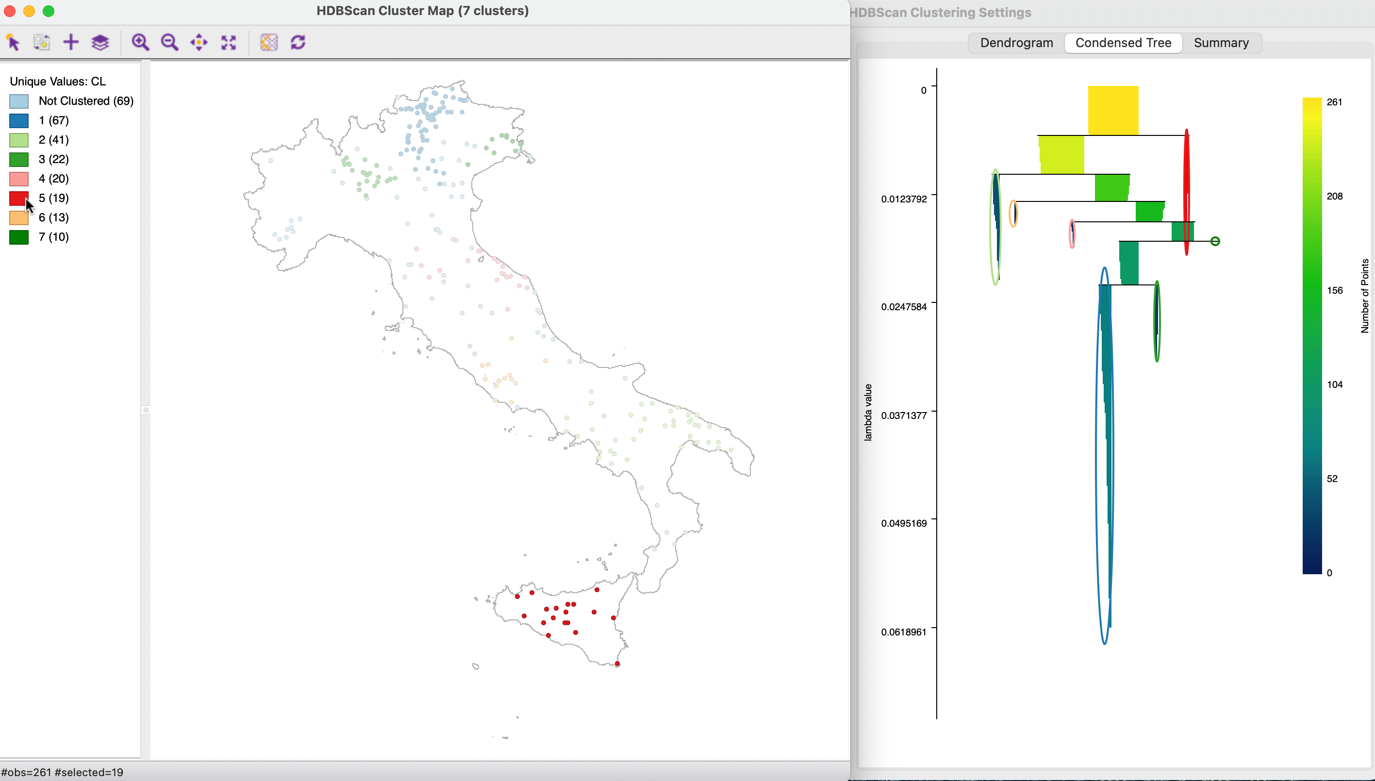
Figure 20.20: HDBSCAN Condensed Tree

In GeoDa, the condensed tree supports linking and brushing as well as a limited form of zoom operations. The latter may be necessary for larger data sets, where the detail is difficult to distinguish in the overall tree. Zooming is implemented as a specialized mouse scrolling operation, slightly different in each system. For example, on some track pads, this works by moving two fingers up or down. There is no panning, but the focus of the zoom can be moved to specific subsets of the graph.

20.5.5.2 Cluster membership

The Save button provides the option to add the core distance, cluster membership probability and outlier index (GLOSH) to the data table. The default variable names are HDB_CORE for the core distance associated with each point, HDB_PVAL for the degree of cluster membership, and HDB_OUT for the outliers. These variables can be included in any type of map. For example, Figure 20.21 shows the degree of cluster membership as a natural breaks map with 6 intervals. Clearly, the observations near the center of the cluster (smaller core distances) carry a darker color and locations further away from the core, are lightly colored.

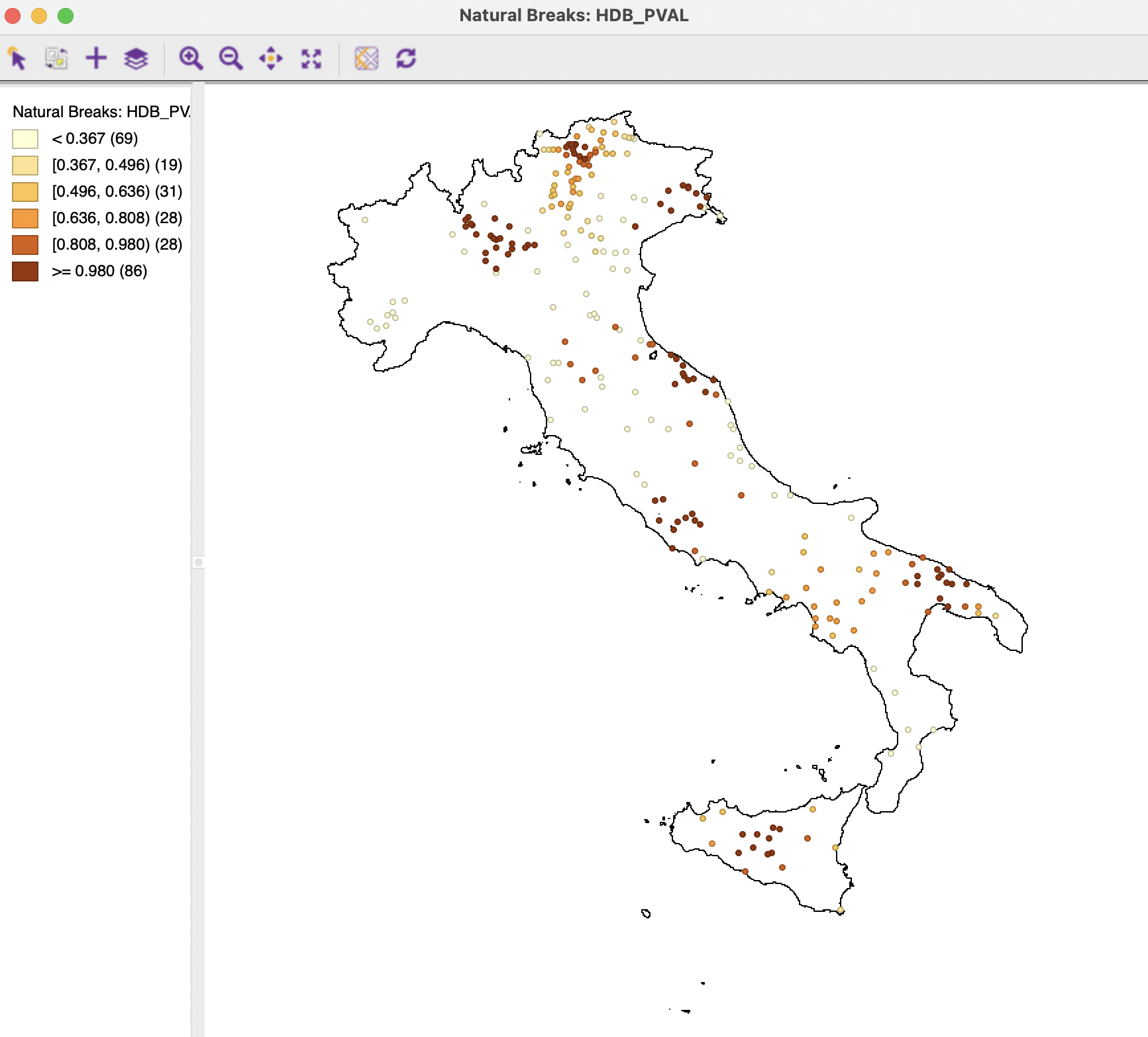
Figure 20.21: HDBSCAN Cluster Membership

A similar map can be created for the outlier probability. This will show the reverse shading, with more remote points colored darker.

20.5.5.3 Core distance map

With the the core distance for each point saved to the data table (HDB_CORE), in GeoDa it is possible to create a Heat Map of the core distances on top of the Cluster Map.¹³³ This is one of the Heat Map options, invoked by right clicking on the cluster point map. The core distance variable must be specified in the Specify Core Distance option. This then yields a heat map as in Figure 20.22, where the core distances associated with each cluster are shown in the corresponding cluster color.

The overall pattern in the figure corresponds to gradations in the cluster membership map.

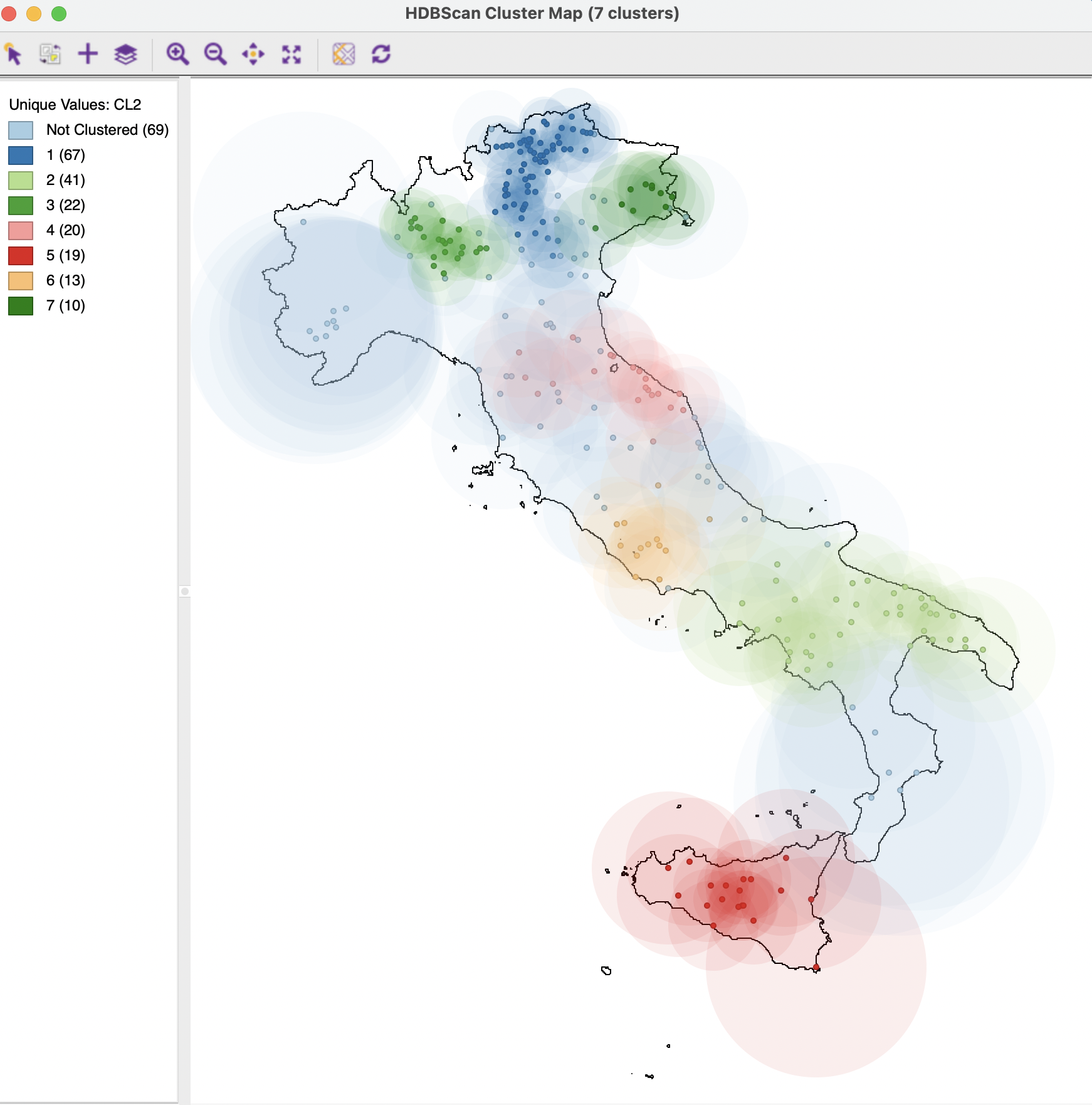
Figure 20.22: HDBSCAN Core Distance Heat Map

---

131. This method is variously referred to as HDBSCAN or HDBSCAN*. Here, for simplicity, the former will be used.↩︎

132. These approaches are sensitive to the influence of the outliers on the estimates of central tendency and spread. This works in two ways. On the one hand, outliers may influence the parameter estimates such that their presence could be masked, e.g., when the estimated variance is larger than the true variance. The reverse effect is called swamping, where observations that are legitimately part of the distribution are made to look like outliers.↩︎

133. Note that for this to work properly, the coordinates used for the point map and the coordinates employed in the HDBSCAN algorithm must be the same. In the current example, this means that COORD_X and COORD_Y should be used instead of their kilometer equivalents. The cluster solutions are the same, since it is a simple rescaling of the coordinates.↩︎