10.3 Creating Contiguity Weigths
In GeoDa, the creation and manipulation of spatial weights is carried out by means of a Weights Manager. This dialog is invoked from the menu as Tools > Weights Manager.
Alternatively, the large W icon on the toolbar can be used, highlighted in
Figure 10.1.
The main interface is shown in Figure 10.9. It contains buttons to Create, Load and Remove weights that are listed under Weights Name. The highlighted weight is the currently active one (for example, see Figure 10.11). Its summary characteristics are listed in the table with columns Property and Value.
A second row of buttons allows various operations on existing weights, including Intersection, Union, and Make Symmetric. Finally, at the bottom of the interface are options to visualize the properties of the weights, in the form of a Histogram, Connectivity Map and Connectivity Graph.
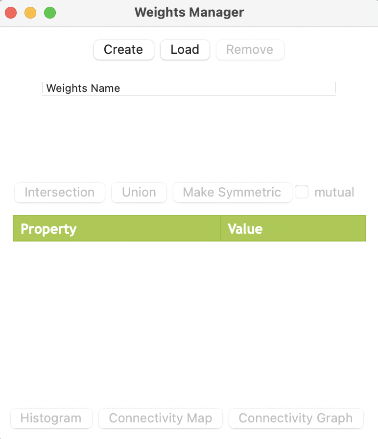
Figure 10.9: Weights Manager interface
10.3.1 Weights manager
The actual construction of the weights is implemented through the Weights File Creation interface, invoked by the Create button. It is shown in Figure 10.10 for the Ceará Zika sample data set. The interface provides the entry point to all the available options. Two buttons correspond to the main types, Contiguity Weight or Distance Weight. In this example, the option for Rook contiguity is checked, with the Contiguity Weight button active.
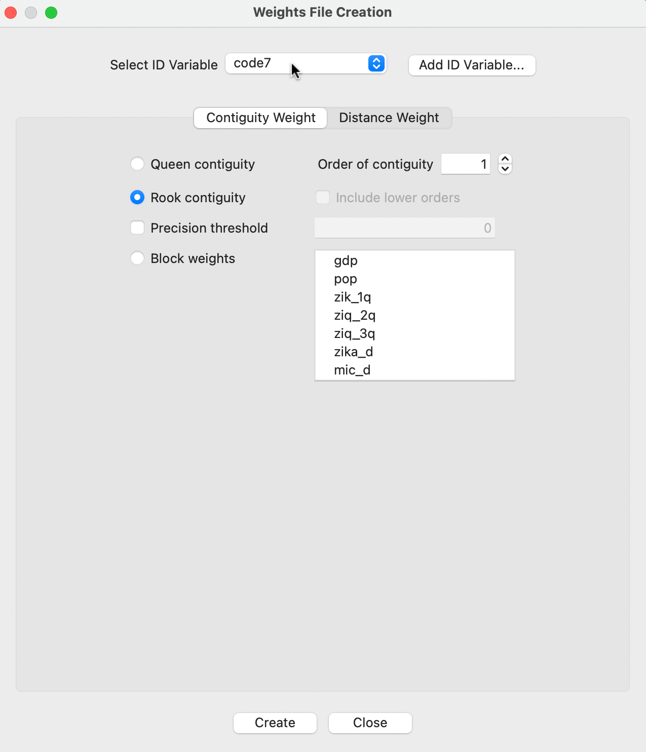
Figure 10.10: Rook contiguity in the Weights File Creation interface
10.3.1.1 ID variable
The first item to specify in the dialog is the ID Variable. This variable has to be unique for each observation. It is a critical element to make sure that the weights are connected to the correct observations in the data table. In other words, the ID variable is a so-called key that links the data to the weights.
In GeoDa, it is best to have the ID Variable be integer. In practice, this is often not the case, and
even though the identifier may look like an integer value, it may be stored as a string. For
example, the standard identifiers that come with many open data sets (such as the US census data) are typically character variables. One way to deal with this problem is to use the Edit Variable Properties functionality in the table to turn a string into an integer, as shown in Section 2.4.1.1.
In some instances, there is no easy way to identify an ID variable. In that case, the Add ID Variable button provides a solution: the added ID variable is simply an integer sequence number that is inserted into the data table (as always, there must be a Save operation to make the addition permanent).
For the Ceará Zika data set, code7 is used as the ID variable, as indicated in Figure 10.10.
10.3.2 Rook contiguity
With the Rook contiguity radio button checked, as in Figure 10.10, a click on Create will start the weights construction process.
First, a file dialog appears in which a file name for the weights must be specified (the file extension GAL is added automatically). In the example, this file is ceara_r.gal. Since there are no real metadata in a spatial weights file, it is a good practice to make the file name something meaningful, so that one can remember what type of weight was created. For example, an _r added to the name of the data would suggest rook weights. However, as outlined in Section 10.3.5, if a Project File is saved, several of the characteristics of the weights (i.e., its metadata) are stored in that file for later reuse.
The weights are immediately computed and written to the GAL file. At the end of this operation, a success message appears (or an Error message if something went wrong).
A useful option in the weights file creation dialog is the specification of a Precision threshold (situated right below the Rook contiguity radio button). In most cases, this is not needed, but in some instances the precision of the underlying shape file is insufficient to allow for an exact match of coordinates (to determine which polygons are neighbors). When this happens, GeoDa suggests a default error band to allow for a fuzzy comparison. In most cases,
this will be sufficient to fix the problem.
After the weights are created, the weights manager becomes populated, as shown in Figure 10.11. The name for the file that was just created is now included under the Weights Name. In addition, under the item Property, several summary characteristics are listed. This is further examined in Section 10.4.1.
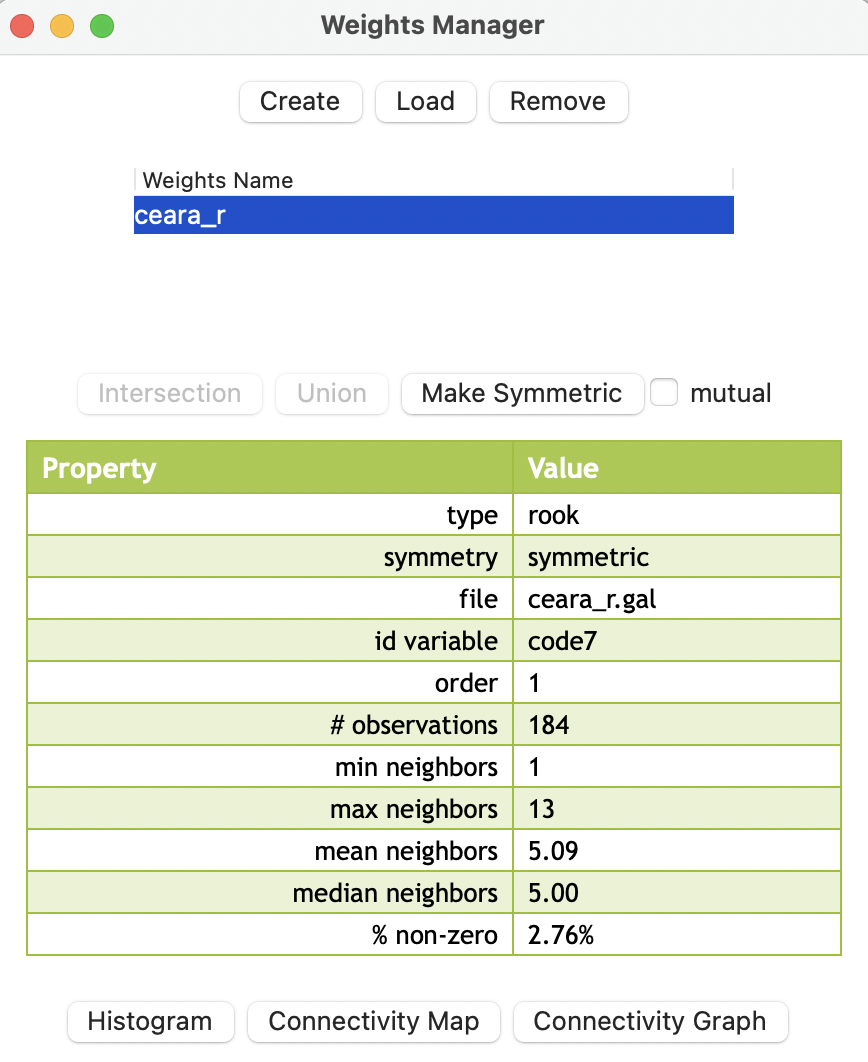
Figure 10.11: Rook weights summary interface
10.3.2.1 GAL file
The GAL weights file is a simple text file that contains, for each observation, the number of neighbors and their identifiers. The format was suggested in the 1980s by the Geometric Algorithms Lab at Nottingham University. It achieved widespread use after its inclusion in SpaceStat (Anselin 1992), and subsequent adoption by the R spdep package and others.
The one innovation SpaceStat added to the format was the inclusion of a header line, with some metadata for the weights, such as the number of observations (184), the name of the shape file from which the weights were derived (zika_ceara), and the name of the ID variable (code7).71 As illustrated in Figure 10.12, for each observation, the number of neighbors is listed after its ID.
For example, for the municipality with code7 2300101, there are 3 neighbors, with
respective IDs 2302503, 2308302, and 2308401.
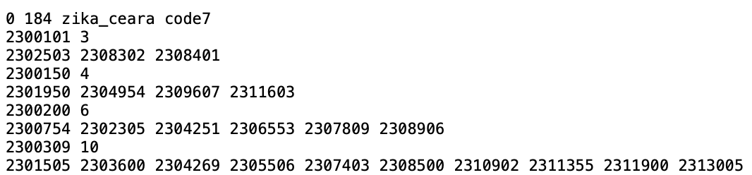
Figure 10.12: GAL file contents
Since the GAL file is a simple text file, it can easily be edited (e.g., to add or remove neighbors), although this is not recommended: it is easy to break the inherent symmetry of the contiguity weights.
10.3.3 Queen contiguity
Spatial weights based on the queen contiguity criterion are created in the same way, but with the Queen contiguity button checked in the dialog of Figure 10.10. If needed, the Precision threshold option is available as well.
After the weights file is created, e.g., ceara_q.gal, its summary properties are listed in the weights manager, with the associated file name highlighted, as in Figure 10.13.
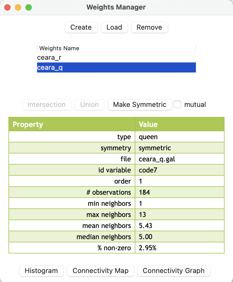
Figure 10.13: Summary properties of first order queen contiguity
10.3.4 Higher order contiguity
Higher order contiguity weights are constructed in the same general manner as the first order weights just considered. To accomplish this, a value larger than the default of 1 must be specified in the Order of contiguity box in Figure 10.10.
One important aspect of higher order contiguity weights is whether or not the lower order neighbors should be included in the weights structure. This is determined by a check box.
Importantly, as outlined in Section 10.2.3, there is a difference between the two concepts. The pure higher order contiguity does not include any lower order neighbors, whereas they are included when the corresponding check box is checked.
Using the second order for the queen contiguity criterion in the Ceará data, e.g., saved into ceara_q2.gal, the summary properties are shown in Figure 10.14.
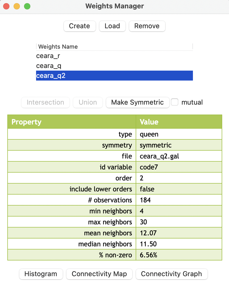
Figure 10.14: Summary properties of second order queen contiguity
In contrast, an encompassing notion of second order neighbors would include the first order neighbors as well. The properties of such a weights file, e.g., ceara_q2i.gal, are listed in Figure 10.15. Note how the include lower orders entry is set to true, in contrast with the entry in Figure 10.14, where it is set to false.
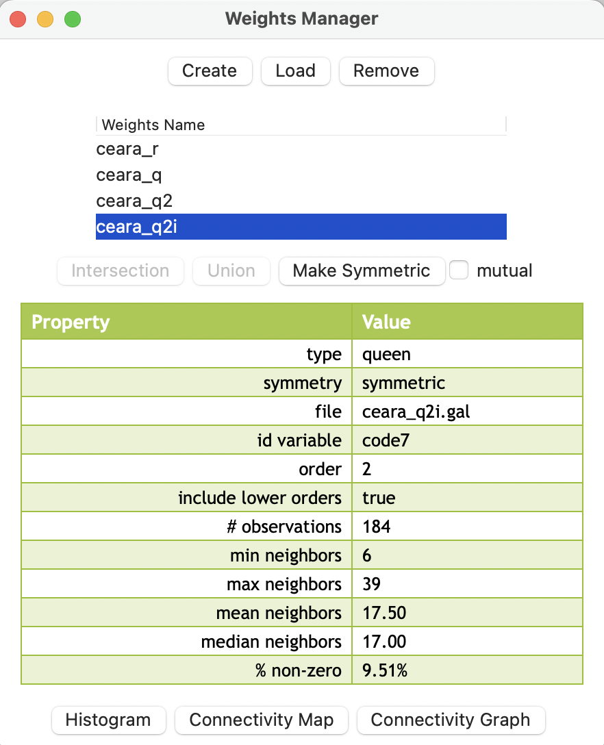
Figure 10.15: Summary properties of second order queen contiguity
The difference between the two concepts can be easily gathered from the descriptive statistics. As expected, the inclusive second order weights are denser. For example, this is illustrated by the percent non-zero: 6.56% for the pure second order, and 9.51% for the inclusive second order. Weights characteristics are considered in more detail in Section 10.4.
10.3.5 Project file
Similar to how custom classifications and grouped variable specifications were earlier saved to a Project File, the same can be achieved for spatial weights. This is very important, since otherwise any weights metadata are lost. They are not included in the saved weights file (see Section 10.3.6).
As before, this is accomplished by invoking File > Save Project and specifying a file name. A gda file extension will be added.
In Figure 10.16, the respective summary weights properties are listed under the weights_entries tag in the file.
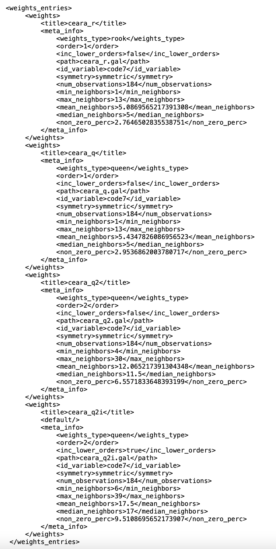
Figure 10.16: Weights description in Project File
As in the previous cases, the gda file must be specified as the input file when starting a new analysis, to make sure the weights are loaded properly. Their properties will immediately appear in the weights manager dialog.
10.3.6 Using Existing Weights
When a Project File is not used as the input, several of the summary properties of the weights are lost. For example, when using the Load option in the weights manager (the middle button in Figure 10.9) for the second order queen contiguity file ceara_q2.gal, the resulting summary is as in Figure 10.17.
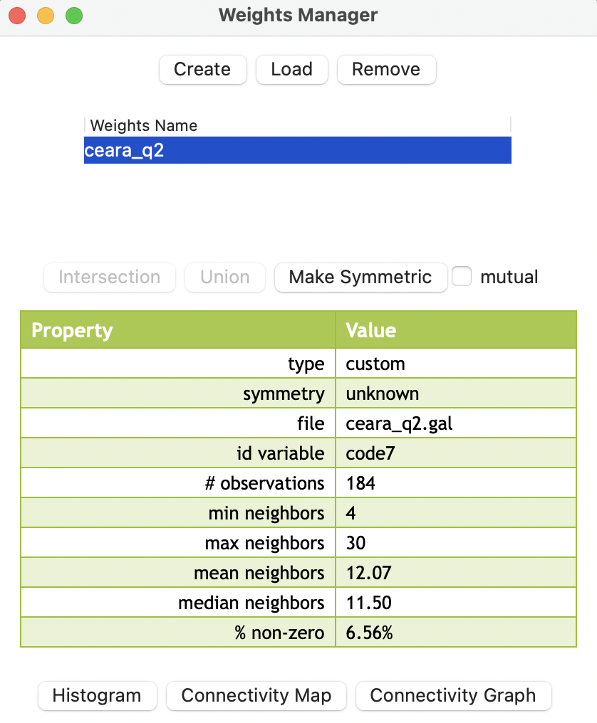
Figure 10.17: Second order contiguity weights loaded from file
In contrast to the entries in Figure 10.14, there is no awareness of the type (set to custom compared to queen), the symmetry, or order of contiguity. Since the numerical properties are computed on the fly, they are still included.
In general, it is highly recommended to use project files to keep track of the spatial weights metadata.
10.3.7 Space-Time weights
The Time Editor considered in Chapter 9, as depicted in Figure 9.2, contains a button in the lower right corner to Save Space-Time Table/Weights.
This is useful in order to trick the cross-sectional data structure of GeoDa to allow for simple pooled time series/cross section analyses.72 The pooled aspect means that the same coefficients or model parameters hold for all time periods, which is not necessarily a realistic assumption. However, it is often the point of departure in an analysis of space-time dynamics.
The critical element in this endeavor is to create a unique space-time ID variable (STID) so that the stacked cross-sections (one for each time period) can be handled as if they were one single cross-sectional data set, with a unique ID for each space-time observation. Analogously, the spatial weights are block-diagonal, with the same weights structure repeated for each stacked time period.
This is illustrated for the Oaxaca Development data set from Chapter 9. Note that it is necessary to have a spatial weights file active in the weights manager for this to work properly. In the example, this is a first order queen contiguity weights file using mun as the ID. A snapshot of the corresponding space-time data table, saved as a csv file, is shown in Figure 10.18. In addition to the cross-sectional identifier mun, there is a unique space-time identifier STID, as well as an indicator variable for each time period: T_2000, T_2010, and T_2020. The remaining entries consist of the time-enabled (grouped) variables.
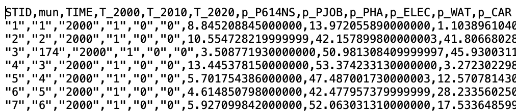
Figure 10.18: Saved space-time table as csv file
The contents of the corresponding gal file are illustrated in Figure 10.19. The header line lists 1710 as the number of space-time observations (\(570 \times 3\)), stoaxaca as the name of the source file with the data (i.e., the file shown in Figure 10.18), and STID as the key. The remaining entries follow the same format as before.
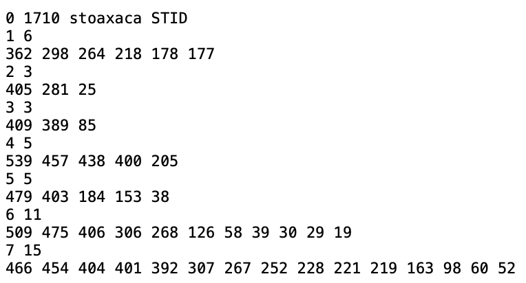
Figure 10.19: Space-time GAL contiguity file