14.2 Specialized Moran Scatter Plots
In this section, two special applications of the Moran scatter plot principle are considered. Each pertains to a different type of situation, both commonly encountered in practice.
In the first example, the data for the same variable are available at different points in time. Rather than having to explicitly compute change values between two points in time, the differential Moran scatter plot provides a short cut, in the sense that the differences are computed under the hood, as part of the scatter plot construction.
The second situation is the familiar case where the variable of interest is a rate or proportion. As discussed at length in Chapter 6, the inherent variance instability of such data is something that needs to be accounted for. This is especially important in the context of spatial autocorrelation, since an important requirement for such statistics to be valid, like Moran’s I, is to have a constant variance. The Morans’ I with EB Rate implements the necessary standardization.
14.2.1 Differential Moran scatter plot
The differential Moran scatter plot is a short cut to compute Moran’s I for the first difference of a variable measured at two points in time. Specifically, for a variable \(y\) observed for each location \(i\) at times \(t\) and \(t-1\), the spatial autocorrelation coefficient is computed for the difference \(y_{i,t} - y_{i,t-1}\).
The difference operation takes care of any temporal correlation that may be the result of a spatial fixed effect, i.e., one or more variables determining the value of \(y_i\) that remain unchanged over time. Examples of such fixed effects are locational advantages (e.g., a port city), or regulatory differences (state income tax vs. no income tax).
More formally, with \(\mu_i\) as the spatial fixed effect associated with location \(i\), the value at each location for times \(t\) and \(t-1\) can be expressed as the sum of some intrinsic value \(u\) and the fixed effect: \[y_{i,t} = u_{i,t} + \mu_i,\] and \[y_{i,t-1} = u_{i,t-1} + \mu_i,\] where \(\mu_i\) is unchanged over time (hence, fixed).
The presence of \(\mu_i\) in both time periods induces a temporal correlation between \(y_{i,t}\) and \(y_{i,t-1}\), above and beyond the intrinsic correlation between \(u_{i,t}\) and \(u_{i,t-1}\). Even when \(u_{i,t}\) and \(u_{i,t-1}\) are uncorrelated, the correlation between \(y_{i,t}\) and \(y_{i,t-1}\) would be E\([\mu_i^2]\), or the variance of the fixed effect.
Taking the first difference eliminates the fixed effect and ensures that any remaining correlation is solely due to \(u\): \[y_{i,t} - y_{i,t-1} = u_{i,t} + \mu_i - u_{i,t-1} - \mu_i = u_{i,t} - u_{i,t-1}.\]
A differential Moran’s I is then the slope in a regression of the spatial lag of the difference, i.e., \(\sum_j w_{ij} (y_{j,t} - y_{j,t-1})\) on the difference \((y_{i,t} - y_{i,t-1})\).
In GeoDa, the slope computation is applied
to the standardized value of the difference (i.e., the
standardization of \(y_{i,t} - y_{i,t-1}\)), and not to the difference between the standardized values.
14.2.1.1 Implementation
The differential Moran scatter plot functionality is the third item in the drop down list activated by the Moran scatter plot toolbar icon (Figure 13.1). Alternatively, it can be started from the main menu as Space > Differential Moran’s I.
Note that this option is only available for data sets with grouped variables (see Section 9.2.1). Without grouped variables, a warning message is generated.
The functionality is illustrated with a time enabled version of the Oaxaca Development sample data set (see Chapter 9). The relevant variables include p_P614NS, p_JOB, and p_PHA, among others.
Before proceeding with the actual differential Moran graph, Figure 14.1 illustrates the spatial pattern of access to health care in 2010 and 2020, p_PHA, as box maps.103 The classification is relative and therefore does not reflect that the values for access to health care have improved rather dramatically between these two years: for example, the mean changed from 53.4 % to 75.8 %. The spatial distribution shows some differences, especially in the center of the map, where several municipalities moved from a higher quartile (brown) to a lower quarter (blue), including 14 lower outliers in 2020.
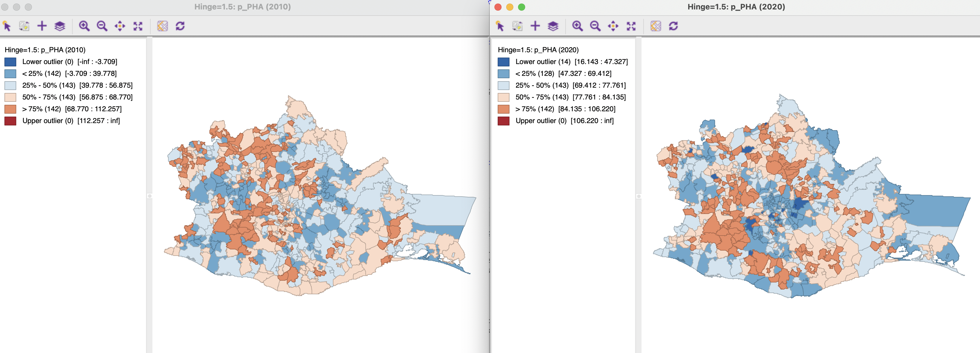
Figure 14.1: Access to health care in 2010 and 2020
A box map for the first difference between 2020 and 2010 (computed in the Table) is shown as Figure 14.2. In contrast to the map for the individual years, the first differences include both lower (2) and upper outliers (8), i.e., areas that improved much less or much more than others, relatively speaking. It is for this spatial pattern that the differential Moran’s I is computed.
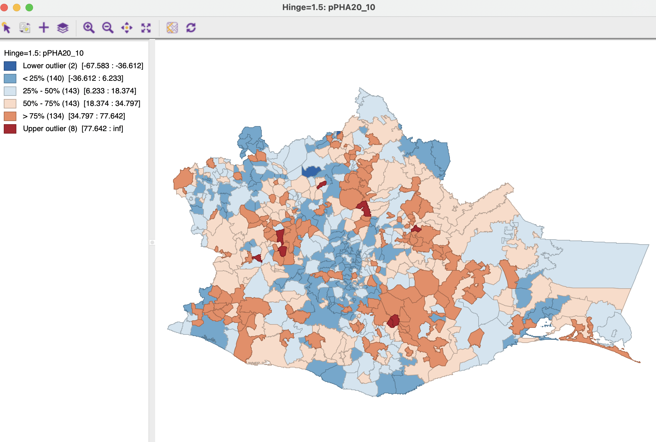
Figure 14.2: Change in access to health care between 2010 and 2020
To provide some context, the individual Moran scatter plots for p_PHA in 2010 and 2020 are shown in Figure 14.3, computed using queen contiguity weights (Oaxaca_q.gal). Both Moran’s I statistics are positive and highly significant, suggesting strong clustering. For 2010, the statistic is 0.221, with an associated z-value of 8.371, for 2020, it is 0.286, with an associated z-value of 11.058. Using 999 permutations, both cases yield a pseudo p-value of 0.001.
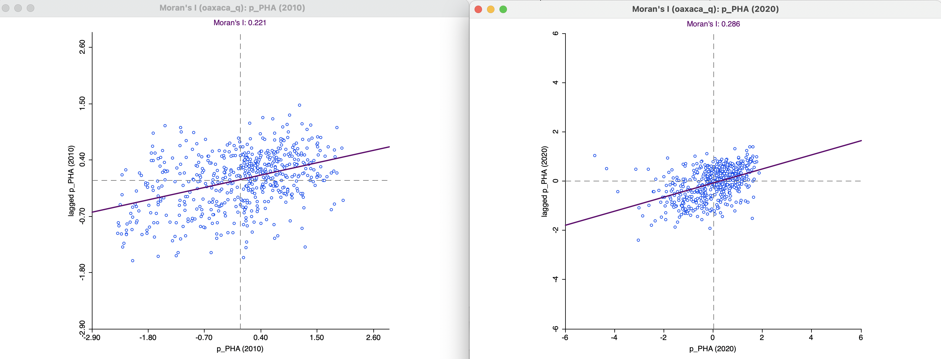
Figure 14.3: Moran scatter plot for access to health care in 2010 and 2020
After starting the differential Moran’s I functionality, a Differential Moran Variable Settings interface provides the means to select the variable and time interval. The drop down list by Select variable contains only the grouped variables in the data set, such as p_PHA for the example. Next, two time periods need to be selected. The values for the time periods are determined by their definition in the Time Editor (see Section 9.2.1). For the illustration, the years 2020 and 2010 are selected (in this order). Finally, the Weights drop down list contains the available spatial weights, here using oaxaca_q.
The resulting differential Moran scatter plot is shown in Figure 14.4. Moran’s I is 0.279, with an associated z-value of 10.611 (from a randomization), again suggesting a strong pattern of clustering. In other words, not only is there clustering in the values of the percent health access, there is also clustering in their change over the ten year period. However, the global Moran’s I provides no information as to where the clustering may happen, nor whether it is driven by high or by low values. This is a common misinterpretation of the global Moran’s I statistic.
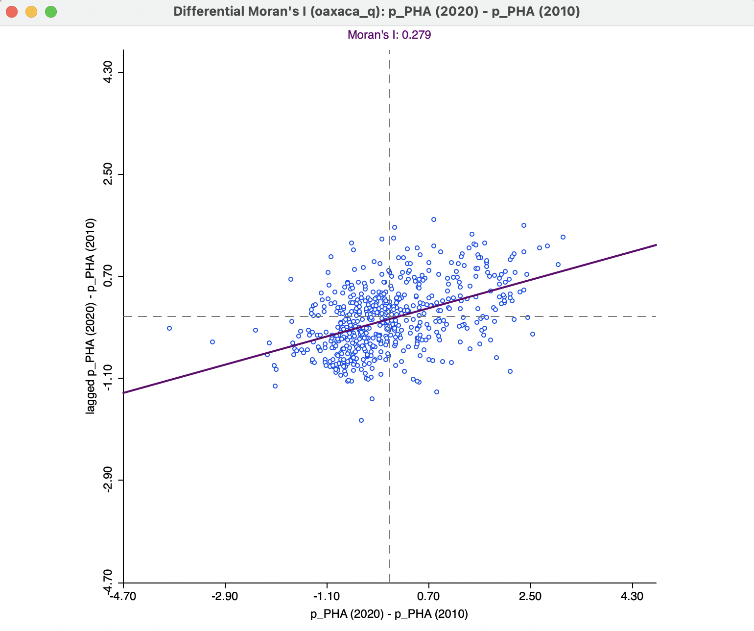
Figure 14.4: Differential Moran scatter plot for access to health care 2020-2010
The differential Moran scatter plot has the same options as the regular Moran scatter plot, with one exception. The Save Results option provides a way to not only save the Standardized Data (as MORAN_STD) and the Spatial Lag (as MORAN_LAG), as in the regular case, but also Diff Values (as DIFF_VAL), the value of the difference before standardization. Clearly, applying a regular Moran scatter plot to this new variable provides the same result as the differential Moran scatter plot. The latter simply saves the effort of first having to construct the differences.
14.2.2 Moran scatter plot for EB rates
In Chapter 6, the issue of the intrinsic variance instability associated with rates or proportions was introduced. The proposed solution was to utilize the Bayesian idea of borrowing strength through various smoothing operations, including an Empirical Bayes (EB) procedure (Section 6.4.2.2).
One may be tempted to carry out spatial autocorrelation tests on EB smoothed rates, but this is not appropriate, since their construction already induces a degree of correlation. Instead, Assunção and Reis (1999) suggested a slightly different procedure to correct Moran’s I spatial autocorrelation test statistic for varying population densities across observational units, when the variable of interest is a rate or proportion. In this approach, the spatial autocorrelation is not computed for a smoothed version of the original rate, but for a transformed standardized random variable. In other words, the crude rate is turned into a new variable that has a constant variance. The mean and variance used in the transformation are computed for each individual observation.
The principle is similar to the shrinkage estimator presented in Section 6.4.2.2, in that it adjusts the crude rate with a mean and variance obtained from a prior distribution. As in the case of EB smoothing, these moments are computed from the data, hence the designation as empirical Bayes.
As before, the point of departure is the crude rate, \(r_i = O_i / P_i\), where \(O_i\) is the count of events at location \(i\) and \(P_i\) is the corresponding population at risk.
The rationale behind the Assunção-Reis approach is to standardize each \(r_i\) as \[z_i = \frac{r_i - \beta}{\sqrt{\alpha + (\beta / P_i)}},\]
using an estimated mean \(\beta\) and standard deviation \(\sqrt{\alpha + \beta / P_i}\). The parameters \(\alpha\) and \(\beta\) are related to the prior distribution for the risk, similar to the treatment in Section 6.4.2.2.
In practice, the prior parameters are estimated by means of the so-called method of moments (e.g., Marshall 1991), yielding the following expressions: \[\beta = O / P,\] with \(O\) as the total event count (\(\sum_i O_i\)), and \(P\) as the total population count (\(\sum_i P_i\)), and \[\alpha = [\sum_i P_i ( r_i - \beta )^2 ] / P - \beta / ( P / n),\]
with \(n\) as the total number of observations (in other words, \(P/n\) is the average population).
One problem with the method of moments estimator
is that the expression for \(\alpha\) could yield a
negative result. In that case, its value is typically set to zero, i.e.,
\(\alpha=0\).
However, in Assunção and Reis (1999), the value for \(\alpha\) is only set to zero
when the resulting estimate for the variance is negative,
that is, when \(\alpha + \beta / P_i < 0\). Slight differences in the
standardized variates may result depending on the convention used. In GeoDa,
when the variance estimate is negative, the original crude rate is used.
Also, after the EB adjustment, the rates are further standardized to have a mean of zero and a variance of one, in the usual fashion for a Moran scatter plot.
14.2.2.1 Implementation
The Moran scatter plot for standardized rates is invoked from the main menu as Space > Moran’s I with EB Rate, or as the fourth item in the drop down list from the Moran scatter plot toolbar icon, Figure 13.1.
To illustrate this procedure, the same disability rate example for Oaxaca municipalities is used as in Section 12.4.0.1, i.e., the ratio of the number of disabled persons (DIS20) over the municipal population (PTOT20) in 2020. The crude rate and EB smoothed rate are mapped in Figure 12.9.
The left panel of Figure 14.5 shows the Moran scatter plot obtained for the crude rate, again using queen contiguity for the spatial weights. The Moran statistic is 0.2649, with an associated z-value (from 999 permutations) of 10.354.
The right hand panel is for the EB Moran scatter plot. This is obtained through the same variable selection interface as for spatially smoothed rates in Section 12.4.1.1, with a variable for the numerator (DIS20) and for the denominator (PTOT20), as well as the spatial weights (oaxaca_q).
The result for the EB Moran’s I is only slightly different from the crude rate, yielding a statistic of 0.2680, with associated z-value of 10.452. However, the values along the horizontal axis show the effect of the standardization, with a much smaller range than for the crude rate.
In practice, the differences between Moran’s I for the crude rate and EB standardized rate tend to be minor.
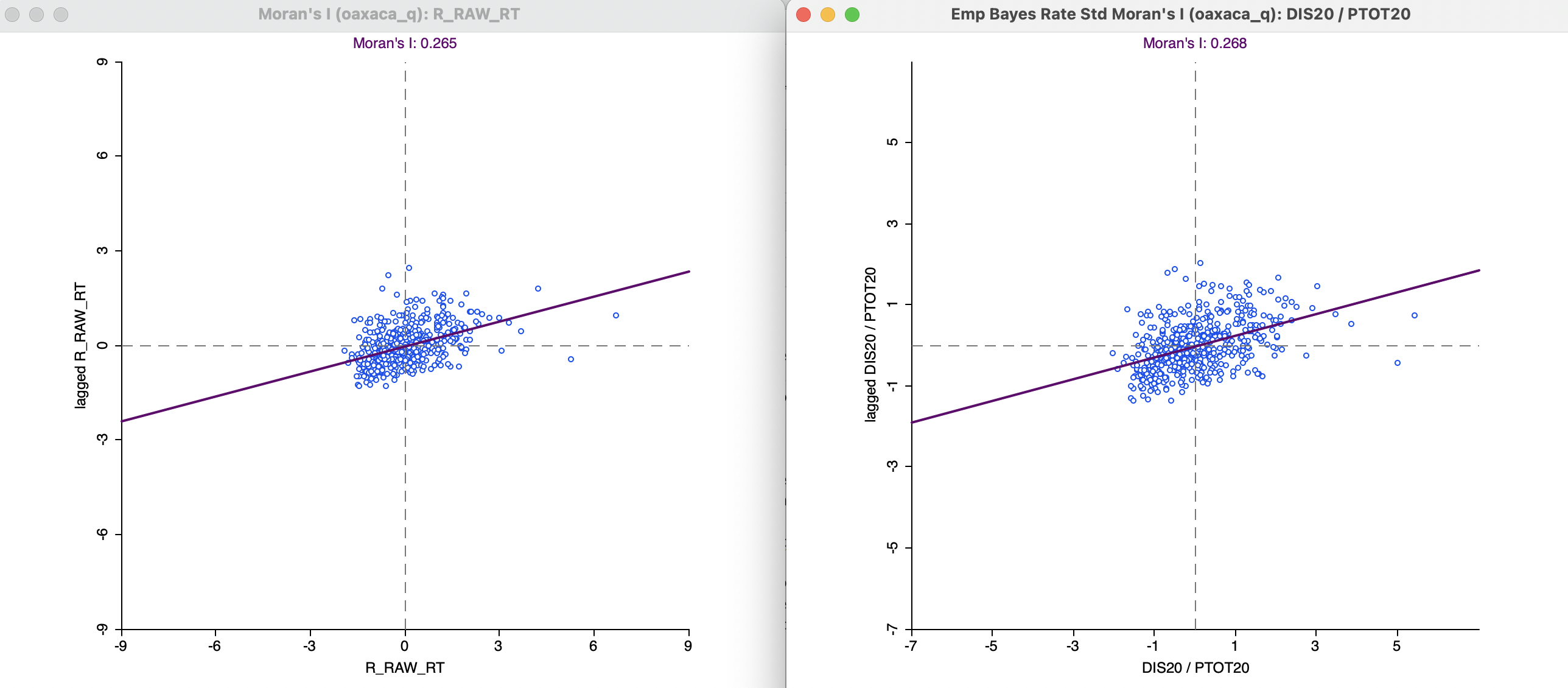
Figure 14.5: Moran scatter plot for raw rate and EB Moran scatter plot
The EB standardized Moran scatter plot has all the same options as the conventional Moran scatter plot, except again for the Save Results feature. In addition to the Standardized Data (the values used in the calculation of the Moran scatter plot), and their Spatial Lag, the EB Rates (i.e., before the standardization used in the Moran computation) can be saved, with default variable name MORAN_EB.
Note that the item in the variable selection list is initially given as p_PHA (all times). After selection, this becomes, respectively, p_PHA (2010) and p_PHA (2020).↩︎