11.5 Broadening the Concept of Contiguity

The concept of contiguity can be generalized to point layers by converting the latter to a tessellation, such as Thiessen polygons (see Section 3.3). Queen or rook contiguity weights can then be created for these polygons, in the usual way.

Similarly, the concepts of distance-band weights and k-nearest neighbor weights can be generalized to polygon layers by considering their centroids (see Section 3.3.1). The polygons are represented by their central points and the standard distance computations are applied.

These operations can be carried out explicitly, by actually creating a separate Thiessen polygon layer or centroid point layer, and subsequently applying the weights operations. However, in GeoDa, this is not necessary, since the computations happen under the hood. In this way, it is possible to create contiguity weights for points or distance weights for polygons directly in the Weights File Creation dialog.

11.5.1 Contiguity-based weights for points

To illustrate the concept of contiguity weights for a point layer, consider the layout of six points depicted in Figure 11.12. The Thiessen polygons are drawn as solid lines. This clearly demonstrates how they are perpendicular to the dashed lines that connect the points. The latter correspond to a queen contiguity relation.

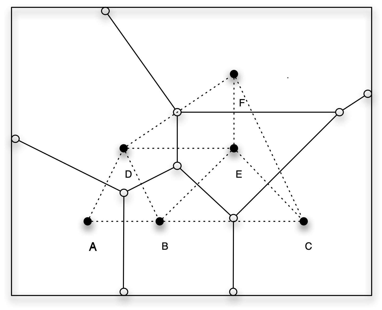
Figure 11.12: Contiguity for points from Thiessen polygons

Contiguity weights for a point layer are created in the same way as such weights for polygon layers. In the Weights File Creation dialog, one selects the Contiguity Weight option and specifies the type of contiguity. For the Italian community bank example, the summary properties of a queen contiguity (italy_banks_te_q.gal) are shown in Figure 11.13.⁷⁹

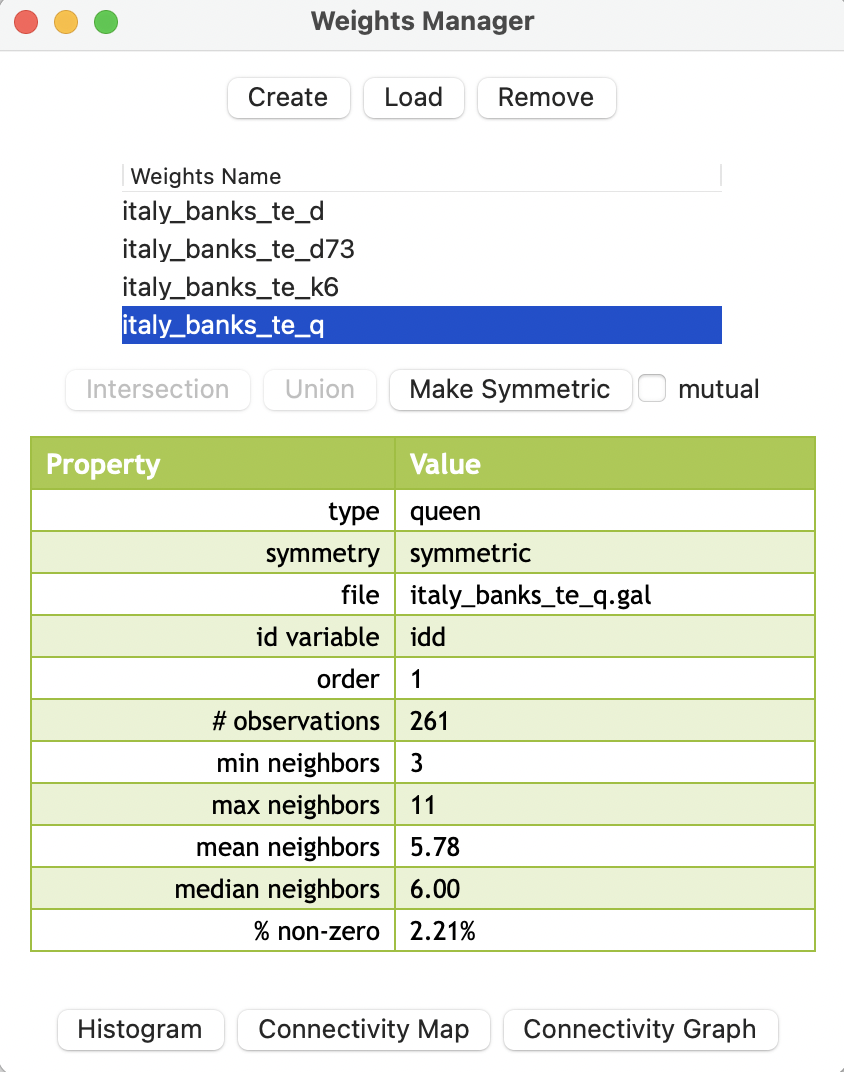
Figure 11.13: Weights summary properties for point contiguity (Thiessen polygons)

Compared to the other weights for this point layer, the mean neighbors is 5.78 and the median neighbors is 6, similar to the k-nearest neighbor results in Figure 11.10. In addition, the resulting weights are still a bit less dense (or, sparser), with a % non-zero of 2.21 % (compared to 2.30 % for k-nearest neighbors).

11.5.1.1 Weights characteristics

These attractive characteristics are also reflected in the connectivity histogram, shown in Figure 11.14. The graph is nicely balanced with a mode of 5-6, near equal to mean and median. There is only a slight skewness to the right.

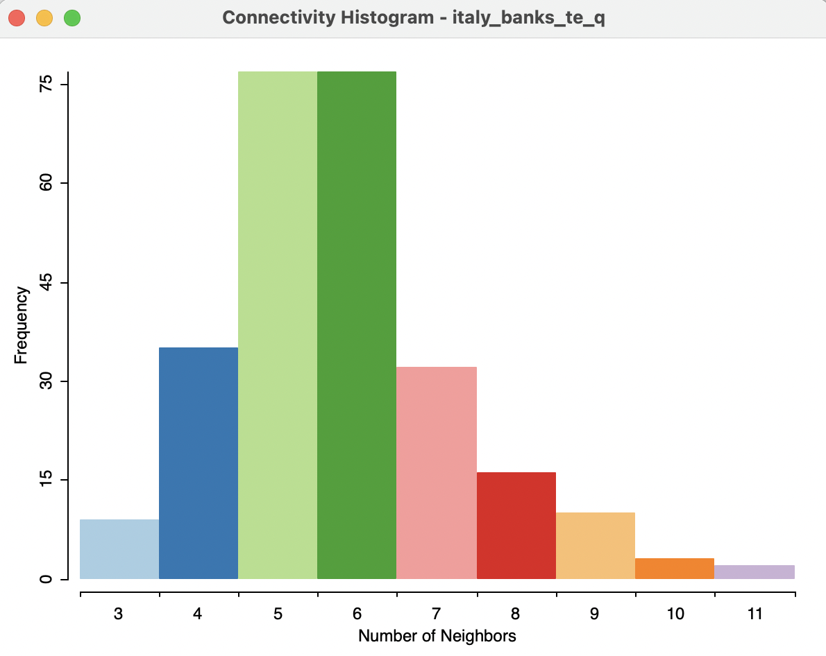
Figure 11.14: Connectivity histogram for point contiguity (Thiessen polygons)

While, at first sight, the queen contiguity weights derived from the Thiessen polygons seem to have attractive properties, there is also a serious drawback. As depicted in Figure 11.15, the Thiessen polygons create several artificial contiguities, making connections between point locations that are totally unrealistic. For example, the connectivity graph shows several links between locations on the island of Sicily and the mainland, crossing the Tyrrhenian Sea. Similarly, a location in Trieste (bordering Slovenia) is connected to several points on the other side of the Adriatic Sea. It is unlikely that these links represent actual interaction between the community banks.

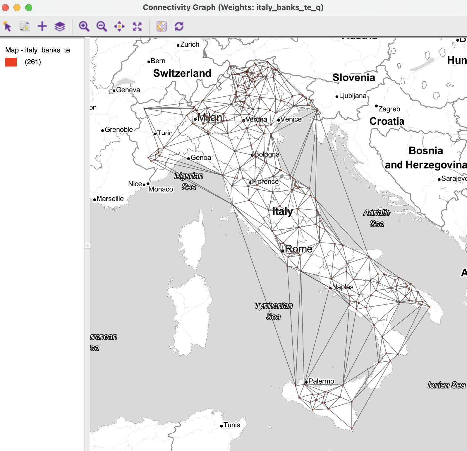
Figure 11.15: Connectivity graph for point contiguity (Thiessen polygons)

A potential solution to this problem is to combine the contiguity weights with other criteria, such as a meaningful distance band, by means of a set operation like intersection (see Section 11.6.1).

11.5.2 Distance-based weights for polygons

As discussed in Section 3.3.1, a polygon layer has a series of Shape Center options to add the centroid or mean center information to the data table, display those points on the map, or save them as a separate point layer. Such points can then be used to construct distance-based weights in the usual way.

However, as is the case for contiguity weights for points, in GeoDa this operation is carried out invisibly, so that it is not necessary to create a separate layer. Distance-band weights and k-nearest neighbor weights are obtained in the same way as for any other point layer (see Section 11.4).

11.5.3 Block weights

A slightly different concept of neighbor follows when a block structure is imposed, in which all observations in the same block are considered to be neighbors. This is a form of hierarchical spatial model, in which all units that share a common higher order level are contiguous.

Familiar examples are counties as part of a state or province, census tracts belonging to a larger neighborhood, etc. In some contexts, the block structure corresponds to the notion of local interaction, in the sense of reflecting the average behavior of a reference group.⁸⁰

The adoption of a block structure became more common in spatial analysis after its application in a study of innovation diffusion by Case (1991).⁸¹ In her study, individual observations on farmers were grouped into districts, and all the farms within the same district were considered to be neighbors. However, the neighbor relation did not extend across districts. In other words, farms that may be physically adjoining but in different districts would not be considered neighbors, in effect turning each district into an island.

The result of this approach is a block-diagonal spatial weights structure. Within each region or district, all observations are neighbors (row elements of 1, except for the diagonal), but there is no neighbor relation between the regions, hence the block-diagonal structure.

The block weights structure has important consequences for the properties of estimators in spatial regression models, but is less useful in an exploratory context, unless used in combination with other criteria.⁸²

11.5.3.1 Weights characteristics

Block weights are invoked as an option of the Contiguity Weight tab in the Weights File Creation dialog. A drop-down list shows potential variables that could be used to define the blocks, as illustrated in Figure 11.16 for the Italian community bank example. In this instance, the variable REGCODE is selected, which provides an integer value for each of the 20 regions in Italy.

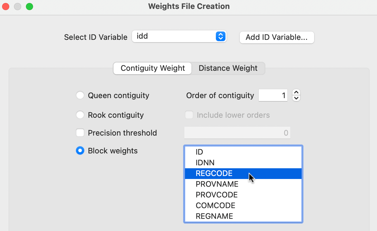
Figure 11.16: Block weights in the Weights File Creation interface

The resulting spatial weights have quite different characteristics. The matrix is not sparse (10.28% non-zero), but not as dense as some distance-band weights. The number of neighbors ranges from 0 (a single observation in a region) to 62. The corresponding graph structure, shown together with the regional boundaries in Figure 11.17, reveals several separate components, with a strong internal connection, but no links between them.⁸³ The sole community bank in the Aosta region is an isolate.

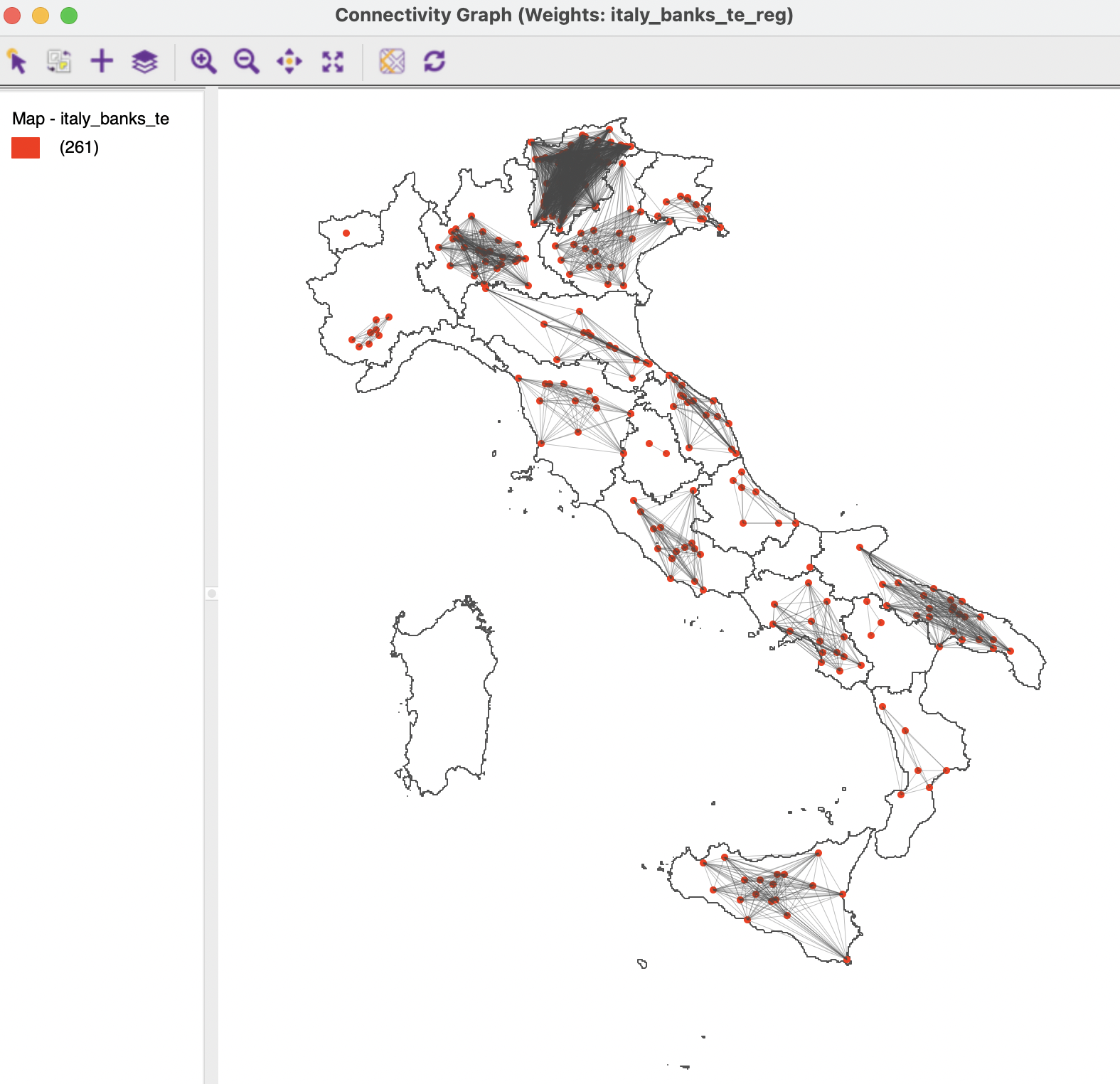
Figure 11.17: Connectivity graph for block weights by region

11.5.4 Space-time weights

A special type of block weights is created as an option of the Time Editor. As mentioned in Section 9.2.1.2, the Save Space-Time Table/Weights button in the interface of Figure 9.2 can generate both a pooled data set as well as a weights file. The latter requires that there is an active weights file in the Weights Manager.

The resulting file follows a GAL format and repeats the cross-sectional contiguity structure for each time period, by using a new space-time index, STID. This index matches the values contained in the corresponding space-time data table. It is a sequential value going from 1 to \(n \times T\), where \(n\) is the cross-sectional dimension and \(T\) is the time dimension.

To illustrate this feature, consider the Oaxaca time-enabled data set from Section 9.2.1 with a first order queen contiguity weights active (oaxaca_q.gal). The contents of the space-time GAL file are illustrated in Figure 11.18.

On the left side, the header line shows how the space-time ID variable, STID takes on values from 1 to 1710 (570 cross-sectional units \(\times\) 3 time periods). The same contiguity structure repeats itself every 570 observations. In the figure, observation 1 has 6 neighbors, with IDs 362, 298, 264, 218, 178, and 177. On the right hand side, observation 571, which corresponds to the first cross-sectional unit in the second time period, has the same six neighbors, but all ID values are incremented by 570. For example, the first neighbor, with STID 932, is obtained as 362 + 570.

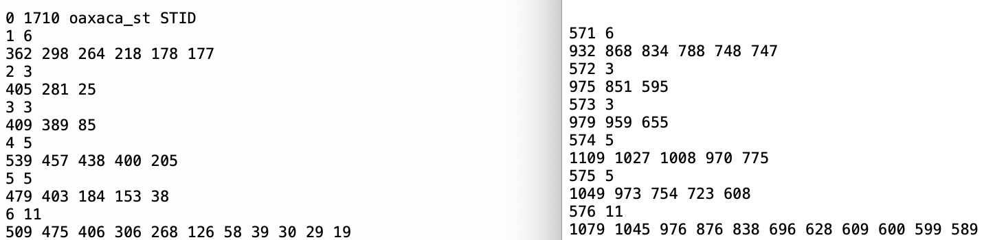
Figure 11.18: Space-time weights GAL file

The resulting space-time weights take on a block-diagonal structure in the sense that the same cross-sectional block repeats itself for each time period. Formally, this corresponds to the matrix expression \(\mathbf{I} \otimes \mathbf{W}\), where \(\mathbf{I}\) is a \(T\)-dimensional identity matrix and \(\mathbf{W}\) are the cross-sectional spatial weights.⁸⁴

The specialized weights structure can be used in a pooled analysis, where the space-time aspect of the data is hidden. The observations are represented as one large cross-section, with variables stacked by time period, and spatial weights block-diagonal by time period. Consequently, all time periods are assumed to have the same parameters, such as the same spatial autocorrelation coefficient.

---

79. Note that the file extension is GAL, as for other contiguity weights.↩︎

80. See, for example, Brock and Durlauf (2001), for a formal discussion.↩︎

81. In some literature, block weights are referred to as Case weights.↩︎

82. For a technical discussion of the spatial econometric aspects, see, e.g., Anselin and Arribas-Bel (2013).↩︎

83. The figure was created by combining the point layer with a polygon layer for the 20 regions, regions.shp, using the multilayer functionality (see Section 3.6).↩︎

84. The symbol \(\otimes\) stands for a Kronecker product. This means that each element of the first matrix is multiplied by the second matrix. In other words, since the first matrix is a \(T \times T\) identity matrix, the result is a block diagonal matrix with a block of \(\mathbf{W}\) for each time period.↩︎