19.3 Bivariate Local Join Count Statistic

In a bivariate binary context, the two variables under consideration, say \(x\) and \(z\), again only take on a value of 0 and 1.

Two different situations are considered, referred to as co-location and no co-location. In the first, it is possible for both variables to take the same value at a location. In other words, at location \(i\), it is possible to have \(x_i = z_i = 1\). For example, this would be the case when the variables pertain to two different types of events that can occur in all locations, such as the presence of several non-exclusive characteristics (e.g., a city block that is both low-density and commercial, or a housing unit that is classified as single family/multifamily and owned/rented).

In the no co-location case, whenever \(x_i = 1\), then \(z_i = 0\) and vice versa. In other words, the two events cannot happen in the same location. This would be case where the classification of a location is exclusive, i.e., if a location is of one type, it cannot be of another type (e.g., majority ethnicity, a zoning classification, or a case-control design). As before, it is important to make sure that the second variable, z, is a rare occurrence, appearing in less than half of the sample.

In GeoDa, the no-colocation case is referred to as Bivariate Local Join Count, since this is the only setting in which it is operational. As conceived, the no co-location setup does not work for more than two variables.

In its general form, the expression for a Bivariate Local Join Count statistic given in Anselin and Li (2019) is: \[BJC_i = x_i (1 - z_i) \sum_j w_{ij} z_j (1 - x_j),\] with \(w_{ij}\) as unstandardized (binary) spatial weights.

The roles of \(x\) and \(z\) may be reversed, but the statistic is not symmetric, so that the results will tend to differ whether \(x\) or \(z\) is the focus. In addition, it is important to keep in mind that the statistic will only be meaningful when the proportion of the second variable (for the neighbors) in the population is small.

Since the condition of no co-location ensures that \(1 - z_i = 0\) whenever \(x_i = 1\), and vice versa, the statistic simplifies to: \[BJC_i = x_i \sum_j w_{ij} z_j,\] whenever \(x_i = 1\), which are the only locations of interest.

Inference can be based on a hypergeometric distribution, considering \(P\) observations with \(x_i = 1\) and \(Q\) observations with \(z_j = 1\). Again, a more robust alternative is based on a permutation approach.

A pseudo p-value can be obtained from a one-sided conditional permutation test. This is implemented by carrying out a series of \(k_i\) draws (with \(k_i\) as the number of neighbors for \(i\)) for each location \(i\) where \(x_i = 1\) (and thus \(z_i = 0\)). The draws are without replacement from \(n-1\) data tuples \((x_j, z_j)\) of which \(Q\) observations have \(z = 1\) (since \(z_i = 0\)) and \(P-1\) observations have \(x = 1\). In practice, we only need to draw the \(z_j\), since the matching \(x_j\) in the tuple are zero by construction. The number of times the resulting local join count statistic equals or exceeds the observed value yields a pseudo p-value, in the usual way.

19.3.1 Implementation

The Bivariate Local Join Count statistic is invoked from the third group in the drop down list associated with the Cluster Maps toolbar icon, or, from the menu, as Space > Bivariate Local Join Count. Next is a Variable Settings dialog from which the two binary variables are selected. The First Variable (X) (\(x\)) is selected from the left-hand column in the dialog, the Second Variable (Y) (\(z\)) is taken from the right-hand column.

Two cases are illustrated in Figure 19.3. In the left-hand panel, the first variable is Hisp with the second variable as Blk. In the right-hand panel, it is the other way around. Both significance maps are based on queen contiguity (Chi_SDOH_q) and use 99,999 permutations with a 0.05 significance cut-off. Clearly, the statistic is not symmetric.

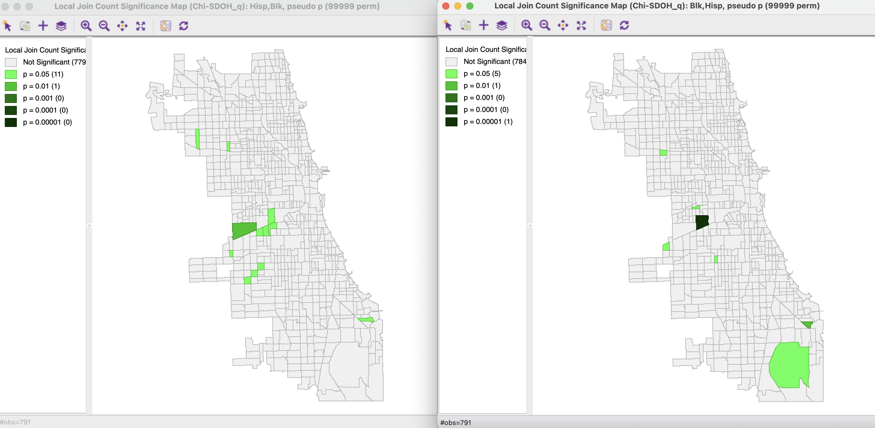
Figure 19.3: Bivariate Local Join Count Significance Map

The statistic picks up the rare occasions where a tract with an ethnic majority of one type is surrounded by tracts with a majority of the other type. In the example, this is only the case in very few instances. Hisp is surrounded by Blk in 12 locations, but 11 of those are only a p = 0.05. Blk is surrounded by Hisp in only 7 instances, but only one of these is highly significant at p < 0.00001. As shown in Figure 19.4, where the neighbors are selected in the unique values map on the left, this is a clear example of a spatial outlier, where a Black majority tract is surrounded by all Hispanic majority tracts.

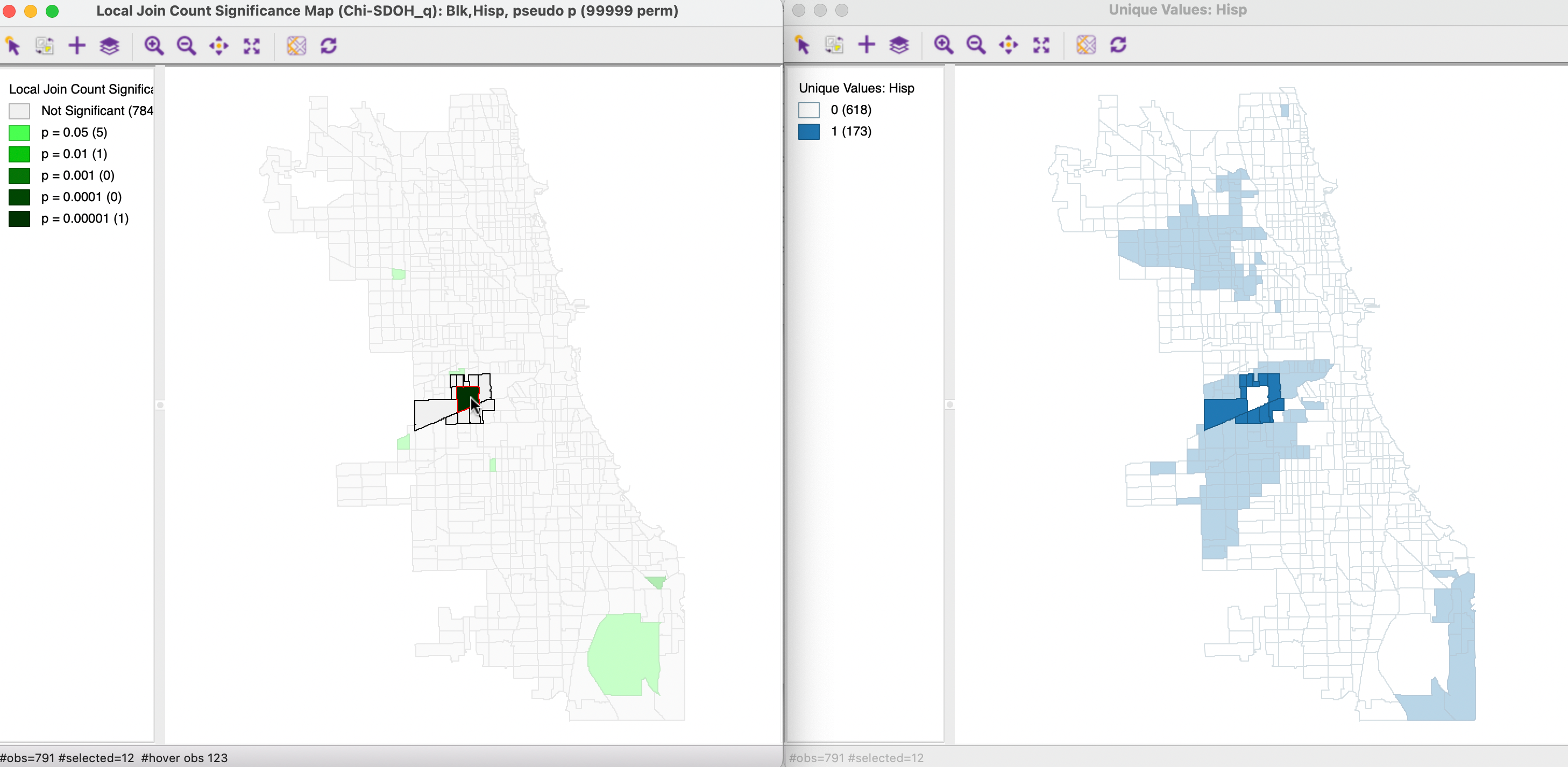
Figure 19.4: Local Join Count Spatial Outlier

All the same options as before are available, including saving the results.