16.5 Significance and Interpretation

The interpretation of the results in a cluster map needs to proceed with caution. Because the permutation test is carried out for each location in turn, the resulting p-values no longer satisfy the classical assumptions. More precisely, because the same data are re-used in several of the tests, the problem is one of multiple comparisons. Moreover, the p-values of the local statistic may be affected by the presence of global spatial autocorrelation, e.g., as investigated by Sokal, Oden, and Thompson (1998b), Ord and Getis (2001), among others. Consequently, the interpretation of the significance of the clusters and outliers is fraught with problems.

In addition, the cluster map only provides an indication of significant centers of a cluster, but the notion of a cluster involves both the core as well as the neighbors.

These issues are considered more closely in the remainder of the current section.

16.5.1 Multiple Comparisons

An important methodological issue associated with the local spatial autocorrelation statistics is the selection of the p-value cut-off to properly reflect the desired Type I error. Not only are the pseudo p-values not analytical, since they are the result of a computational permutation process, but they also suffer from the problem of multiple comparisons (for a detailed discussion, see de Castro and Singer 2006; Anselin 2019a). The bottom line is that a traditional choice of 0.05 is likely to lead to many false positives, i.e., rejections of the null when in fact it holds.

There is no completely satisfactory solution to this problem, and no strategy yields an unequivocal correct p-value. A number of approximations have been suggested in the literature, of which the best known are the Bonferroni bounds and False Discovery Rate approaches. However, in general, the preferred strategy is to carry out an extensive sensitivity analysis, to yield insight into what may be termed interesting locations, rather than significant locations, following the suggestion in Efron and Hastie (2016).

In GeoDa, these strategies are implemented through the Significance Filter option (the second item in the options menu).

16.5.1.1 Adjusting p-values

Adjusting the cut-off p-value as an option of the Significance Filter is straightforward. One can select one of the pre-selected p-values from the list, i.e., 0.05, 0.01, 0.001, or 0.0001. For example, choosing 0.01 immediately changes the locations that are displayed in the significance and cluster maps, as shown in Figures 16.9 and 16.10. The number of significant locations drops from 117 to 47 (for 99,999 permutations), with the 70 observations initially labeled as significant at p < 0.05 removed from the significance map.

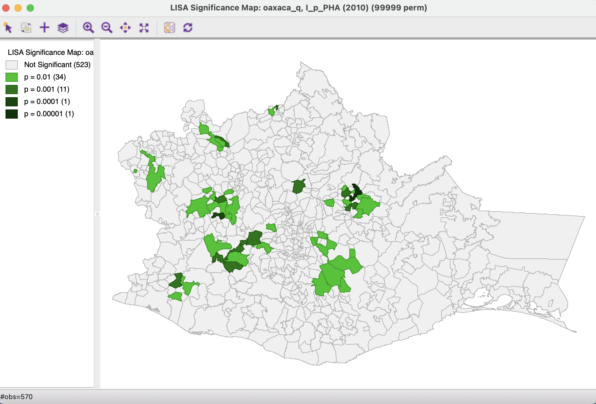
Figure 16.9: Significance map - p < 0.01

Whereas for p < 0.05 the High-High and Low-Low clusters were of comparable size, for p < 0.01 there are almost twice as many Low-Low clusters as High-High. Similarly, for the spatial outliers, which were roughly equally represented for p < 0.05, for p < 0.01 there are more than twice as many High-Low outliers than Low-High outliers.

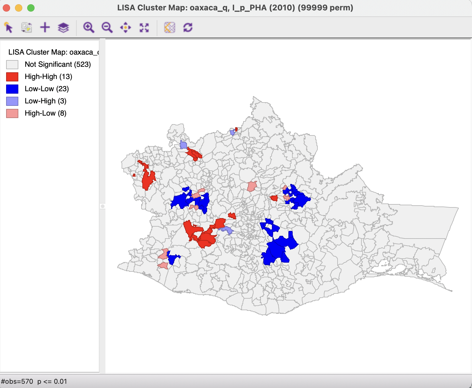
Figure 16.10: Cluster map - p < 0.01

A sensitivity analysis by adjusting the cut-off p-value in this manner provides some insight into which selected clusters and spatial outliers stand up to high scrutiny vs. which are more likely to be spurious.

A more refined approach to select a p-value is available through the Custom Inference item of the significance filter. The associated interface provides a number of options to deal with the multiple comparison problem.

The point of departure is to set a target \(\alpha\) value for an overall Type I error rate. In a multiple comparison context, this is sometimes referred to as the Family Wide Error Rate (FWER). The target rate is selected in the input box next to Input significance. Without any other options, this is the cut-off p-value used to select the observations. For example, this could be set to 0.1, a value suggested by Efron and Hastie (2016) for big data analysis. In the example, this value is kept to the conventional 0.05.

16.5.1.2 Bonferroni bound

The first custom option in the inference settings dialog is the Bonferroni bound procedure. This constructs a bound on the overall p-value by taking \(\alpha\) and dividing it by the number of multiple comparisons. In the LISA context, the latter is typically taken as the number of observations, \(n\), although alternatives have been proposed as well. These include the average or maximum number of neighbors, or some other measure of the range of interaction.

With the number of observations at 570, the Bonferroni bound in the example would be \(\alpha / n = 0.00008772\), the cut-off p-value to be used to determine significance.

Checking the Bonferroni bound radio button in the dialog immediately updates the significance and cluster maps. This typically is a very strict criterion. For example, in the cluster map in Figure 16.11, only two observations meet this criterion, in the sense that their pseudo p-value is less than the cut off.

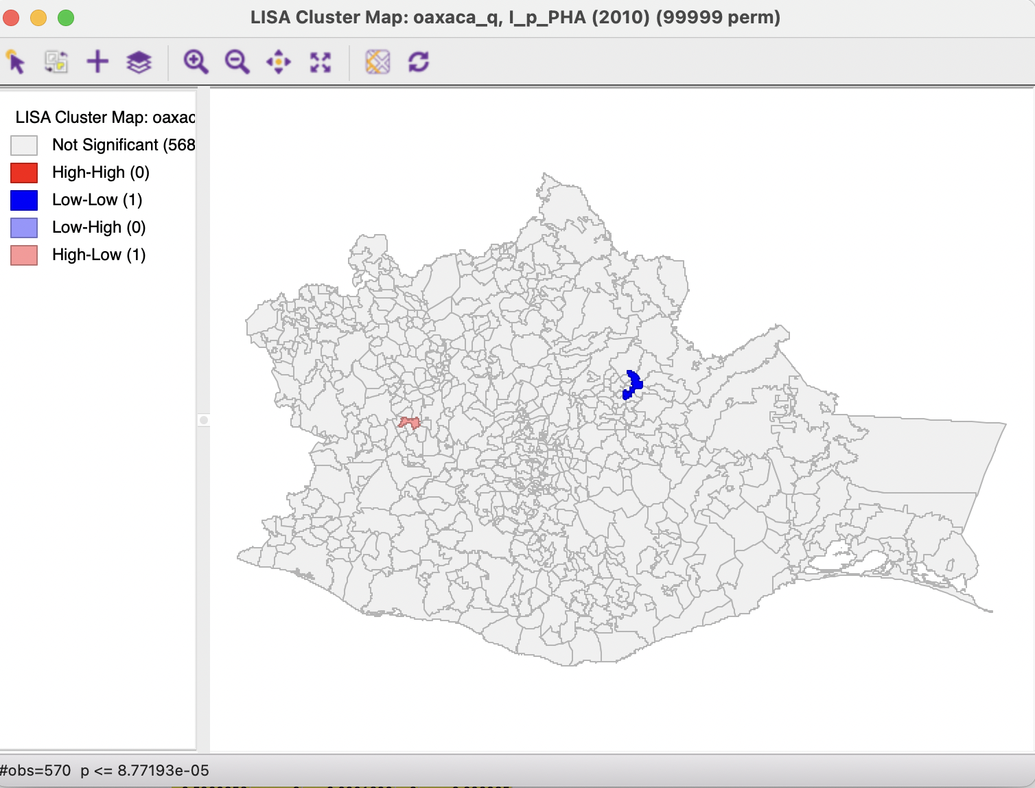
Figure 16.11: Cluster map - Bonferroni bound

16.5.1.3 False Discovery Rate (FDR)

In practice, the application of a Bonferroni bound is often too strict, in that very few (if any) observations turn out to be significant. In part, this is due to the use of the total number of observations as the adjustment factor, which is almost certainly too large, hence the resulting critical p-value will be too small.

A slightly less conservative option is to use the False Discovery Rate (FDR), first proposed by Benjamini and Hochberg (1995). It is based on a ranking of the pseudo p-values from the smallest to the largest. The FDR approach then consists of selecting a cut-off point as the first observation for which the pseudo p-value is not smaller than the product of the rank with \(\alpha / n\). With the sorted order as \(i\), the critical p-value is the value in the sorted list that corresponds with the sequence number \(i_{max}\), the largest value for which \(p_{i_{max}} \leq i \times \alpha / n\).

To illustrate this method, a few additional columns are added to the data table in the example. First, as shown in Figure 16.12, the column LISA_p containing the pseudo p-values is sorted in increasing order (signified by the > symbol next to the variable name). Next, a column with the sorted order is added, as pOrder.¹¹⁴ A new column is added with the FDR reference value. This is the product of the sequence number in pOrder with \(\alpha / n\), which for the first observations is the same as the Bonferroni bound, shown as 0.000087 in the table. The value for the second observation is then \(2 \times 0.000087\) or \(0.000174\).¹¹⁵

The full result is shown in Figure 16.12, with the observations that meet the FDR criterion highlighted in yellow. For the 17th ranked observation (location 55), the pseudo p-value of 0.00139 still meets the criterion of 0.001479, but for the 18th ranked observation, this is no longer the case (0.001730 > 0.001556).

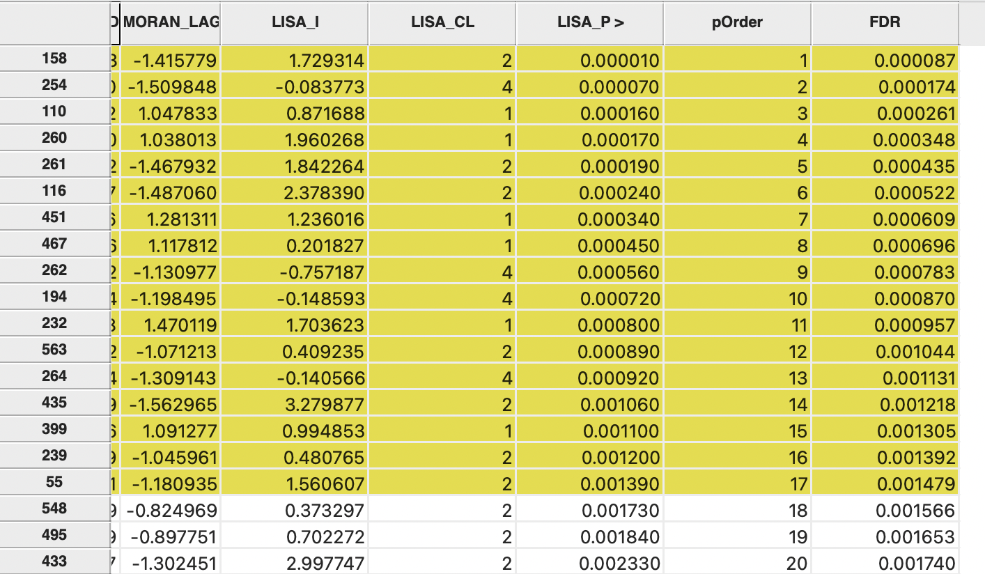
Figure 16.12: False Discovery Rate calculation

Checking the False Discovery Rate radio button will update the significance and cluster maps accordingly, displaying only 17 significant locations, as shown in Figure 16.13. At this point, the High-High and Low-Low clusters are again fairly balanced (respectively, 6 and 7), but there are no longer any Low-High spatial outliers (there are 4 remaining High-Low outliers).

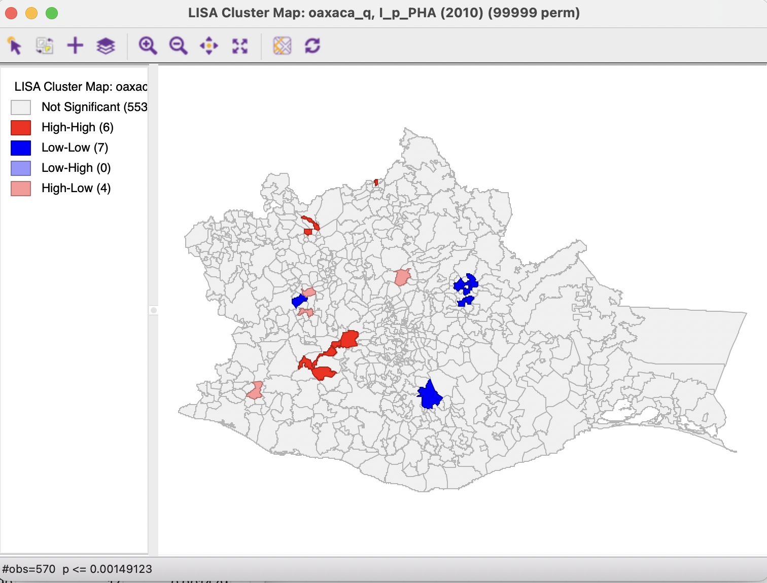
Figure 16.13: Cluster map - FDR

16.5.2 Interpretation of Significance

As mentioned, there is no fully satisfactory solution to deal with the multiple comparison problem. Therefore, it is recommended to carry out a sensitivity analysis and to identify the stage where the results become interesting. A mechanical use of 0.05 as a cut off value is definitely not the proper way to proceed.

Also, for the Bonferroni and FDR procedures to work properly, it is necessary to have a large number of permutations, to ensure that the minimum p-value can be less than \(\alpha / n\). Currently, the largest number of permutations that GeoDa supports is 99,999, and thus the smallest possible p-value is 0.00001. For the Bonferroni bound to be effective, \(\alpha / n\) must be greater than 0.00001, or \(n\) should be less than \(\alpha / 0.00001\). This is not due to a characteristic of the data, but to the lack of sufficient permutations to yield a pseudo p-value that is small enough.

In practice, this means that with \(\alpha = 0.01\), data sets with \(n > 1000\) cannot have a single significant location using the Bonferroni criterion. With \(\alpha = 0.05\), this value increases to 5000, and with \(\alpha = 0.1\) to 10,000.

The same limitation applies to the FRD criterion, since the cut-off for the first sorted observation corresponds with the Bonferroni bound (\(1 \times \alpha/n\)).

Clearly, this drives home the message that a mechanical application of p-values is to be avoided. Instead, a careful sensitivity analysis should be carried out, comparing the locations of clusters and spatial outliers identified for different p-values, including the Bonferroni and FDR criteria, as well as the associated neighbors to suggest interesting locations that may lead to new hypotheses and help to discover the unexpected.

16.5.3 Interpretation of Clusters

Strictly speaking, the locations shown as significant on the significance and cluster maps are not the actual clusters, but the cores of a cluster. In contrast, in the case of spatial outliers, the observations identified are the actual locations of interest.

In order to get a better sense of the spatial extent of the cluster, the Select All… option offers a number of ways to highlight cores, their neighbors, or both.

The first option selects the cores, i.e., all the locations shown as non-white in the map. This is not so much relevant for the cluster or significance map, but rather for any maps that are linked. The selection of the Cores will select the corresponding observations in any other map or graph window.

The next option does not select the cores themselves, but their Neighbors. Again, this is most relevant when used in combination with linked maps or graphs.

The third option selects both the cores and their neighbors (as defined by the spatial weights). This is most useful to assess the spatial range of the areas identified as clusters. For example, in Figure 16.14, the Cores and Neighbors option is applied to the significant locations obtained using the FDR criterion. The non-significant neighbors are shown in grey on the cluster map on the right, with all the matching cores and neighbors highlighted in the box map on the left.

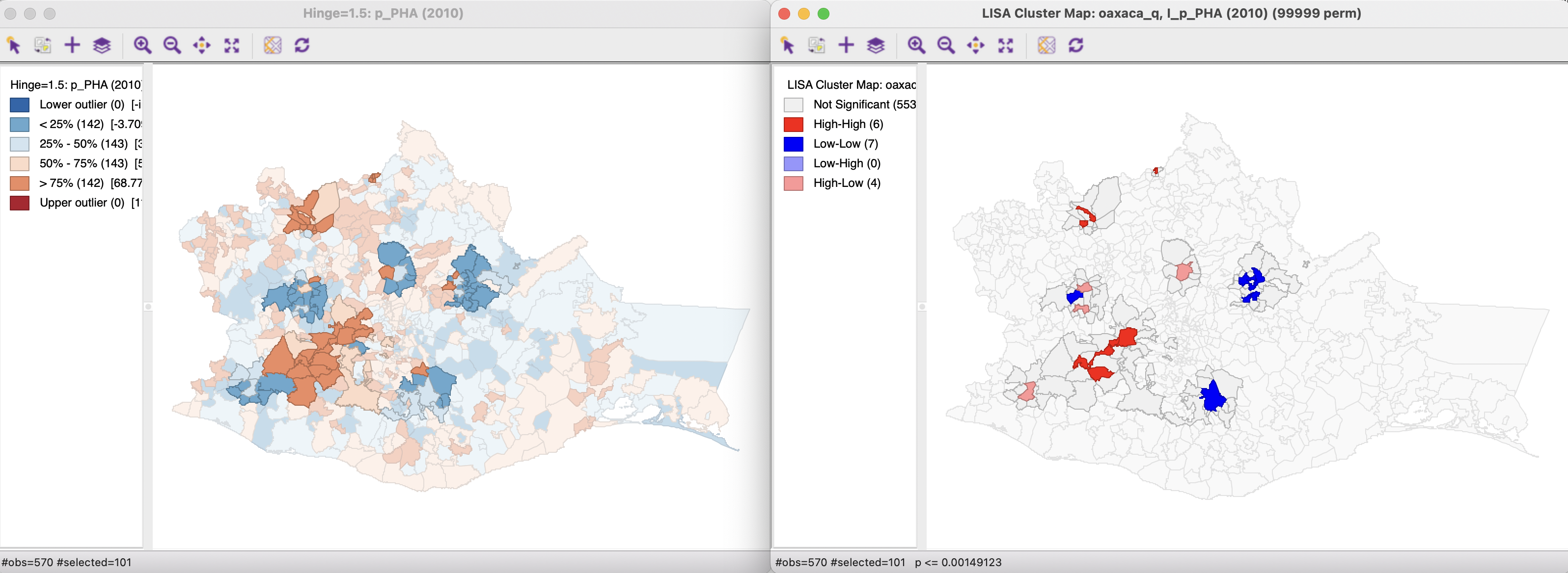
Figure 16.14: Cores and neighbors

A careful application of this approach provides insight into the spatial range of interaction that corresponds with the respective cluster cores.

---

114. This is accomplished by means of the Table Calculator, using Special > Enumerate.↩︎

115. Again, this is accomplished in the Table Calculator. First, the new column/variable FDR is set to the constant value \(\alpha / n\), using Univariate > Assign. Next, the FDR column is multiplied with the value for pOrder, using Bivariate > Multiply.↩︎