19.2 Univariate Local Join Count Statistic
For binary variables, coded as 0 and 1, the global spatial autocorrelation statistic of choice is the join-count statistic (see Cliff and Ord 1973). This statistic consists of counting the joins that correspond to occurrences of value pairs at neighboring locations. The three cases are joins of \(1-1\) (so-called BB joins, for black-black), \(0-0\) (so-called WW joins, for white-white), and \(0-1\) (so-called BW joins). The former two are indicators of positive spatial autocorrelation, the latter of negative spatial autocorrelation.
The primary interest lies in identifying co-occurrences of uncommon events, i.e., situations where observations that take on the value of 1 constitute much less than half of the sample. The definition of what is 1 or 0 can easily be reversed to make sure this condition is met. Therefore, the focus is on the BB join counts. While this is not an absolute requirement, the way the inference is obtained requires that the probability of obtaining a large number of like neighbors is small, and thus can form the basis for rejecting the null hypothesis. When the proportion of observations with 1 is larger than half, then the probability of a small number of neighbors with a value of 1 will be small, which is counter the overall logic.123
With the variable \(x_i\) at location \(i\) taking either the value of 1 or 0, a global BB join count statistic can be written as: \[BB = \sum_i \sum_j w_{ij} x_i x_j,\] where \(w_{ij}\) are the elements of a binary spatial weights matrix. In other words, a join is counted when \(w_{ij} = x_i = x_j = 1\). In all other instances, either when there is a mismatch in \(x\) between \(i\) and \(j\), or a lack of a neighbor relation (\(w_{ij} = 0\)), the term on the right-hand side does not contribute to the double sum.
Following the logic in Anselin (1995), Anselin and Li (2019) recently introduced a local version of the BB join count statistic as: \[BB_i = x_i \sum_j w_{ij}x_j,\] where \(x_{i,j}\) can only take on the values of 1 and 0, and, again, \(w_{ij}\) are the elements of a binary spatial weights matrix (i.e., not row-standardized).
The statistic is only meaningful for those observations where \(x_i = 1\), since for \(x_i = 0\) the result will always equal zero. When \(x_i = 1\), it corresponds to the sum of neighbors for which the value \(x_j = 1\). In this sense, it is similar in spirit to to the local second order analysis for point patterns outlined in Getis (1984) and Getis and Franklin (1987), where the number of points are counted within a given distance \(d\) of an observed point. The distance cut-off \(d\) could readily form the basis for the construction of the spatial weights \(w_{ij}\), which yields the join count statistic as a count of events (points) within the critical distance from a given point (\(x_i = 1\)).
The main difference between the two concepts is the underlying data structure: in the point pattern perspective, the locations themselves are considered to be random, whereas the local join count statistic is based on a lattice perspective. The latter considers a finite set of known locations, for which both events (\(x_i = 1\)) and non-events (\(x_i = 0\)) are observed. In point patterns analysis, one does not know the locations where events might have happened, but did not.
In addition, the local join count statistic also has the same structure as the numerator in the local \(G_i\) statistic of Getis and Ord (1992), when applied to binary observations (and with a binary weights matrix). The numerator in this statistic is \(\sum_j w_{ij} x_j\), which is identical to the multiplier in the local join count statistic. However, the difference between the two statistics is that the local \(G_i\) includes the neighbors with \(x_j = 1\) for all locations, including the ones where \(x_i = 0\). Such observations are ignored in the computation of the local join count statistic as outlined above. In a sense, the local join count statistic could thus be considered a constrained form of the local \(G_i\) statistic, limited to observations where \(x_i = 1\).
Inference can be based on a hypergeometric distribution, or, as before, on a permutation approach. Given a total number of events in the sample of \(n\) observations as \(P\), the magnitude of interest is the number of neighbors of location \(i\) for which \(x_i = 1\), i.e., conditional upon observing 1 at this location. The number of neighbors with \(x_j = 1\) is represented by \(p_i\). The probability of observing exactly \(p_i = p\), conditional upon \(x_i = 1\) follows the hypergeometric distribution for \(n - 1\) data points and \(P - 1\) events: \[\mbox{Prob}[p_i = p | x_i = 1] = \frac{ {{P-1} \choose {p}} { {N - P - 2} \choose {k_i - p} }}{ { {N-1} \choose {k_i}} },\] where \(k_i\) is the number of neighbors for observation \(i\).
Instead, a conditional permutation procedure can be followed to compute a pseudo \(p\)-value, in the usual fashion. This is the preferred approach since the probability given by the previous expression underestimates uncertainty, because it ignores the uncertainty associated with observing \(x_i =1\).
In practice, the permutation approach does not require any parametric assumptions. It is formulated as a classical one-sided hypothesis test against the null hypothesis of spatial randomness. In what follows, only the conditional permutation approach is considered. Further technical details are provided in Anselin and Li (2019).
19.2.1 Implementation
To illustrate the univariate Local Join Count statistic, two variables are considered that correspond to census tracts in Chicago with a predominant ethnic make-up. More precisely, these are the tracts where the Hispanic population makes up more than 50% (Hisp), and the tracts where the majority population is Black (Blk).124 A unique values map for these two variables is given in Figure 19.1. The pattern reveals the strong degree of racial segregation, a well-known characteristics of the population distribution in Chicago.
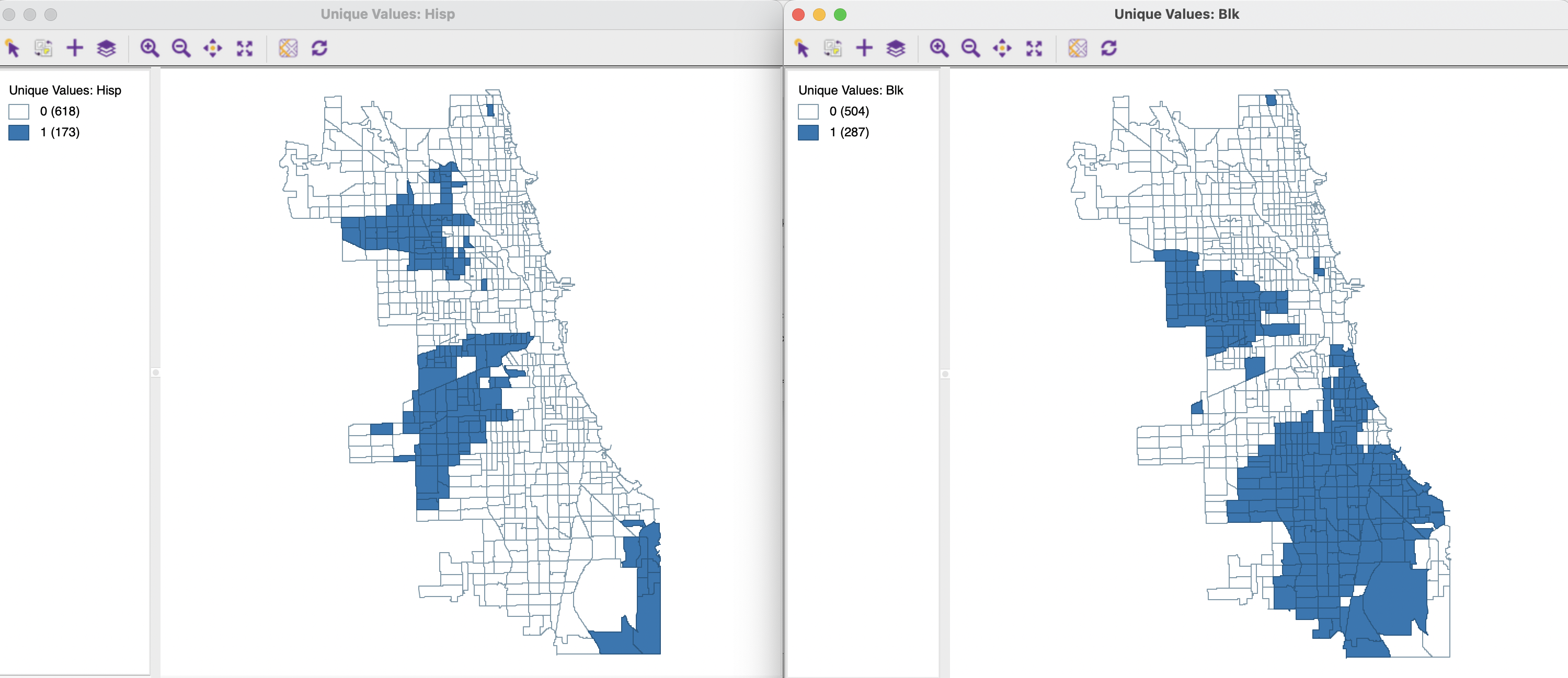
Figure 19.1: Unique Values Black-Hispanic Tracts
The univariate local join count statistic is invoked in the third group in the Cluster Maps drop down list from toolbar icon, or
from the menu, as Space > Univariate Local Join Count. This is followed by a Binary Variable Settings dialog, where the variable is selected and the spatial weights matrix is specified. In this illustration, the spatial weights are queen contiguity (Chi_SDOH_q). This is one of the few instances in GeoDa where the spatial weights are not row-standardized and instead are used as binary weights.
19.2.1.1 Local significance map
The local significance maps for the Univariate Local Join count statistic for respectively Hisp and Blk are shown in the panels of Figure 19.2. The result is for 99,999 permutations and a 0.01 p-value cut-off. The strong impression of local clustering given by the unique values map is confirmed by these significance maps. Unlike what is the case for other local statistics, there is no separate cluster map, since only positive spatial autocorrelation is considered, and there is no notion of High-High or Low-Low. The map shows those cores of clusters with a value of 1 for the variable of interest, where the probability of finding the observed number of neighbors with a value of 1 is highly unlikely. As before, the actual notion of a cluster would include those neighbors.
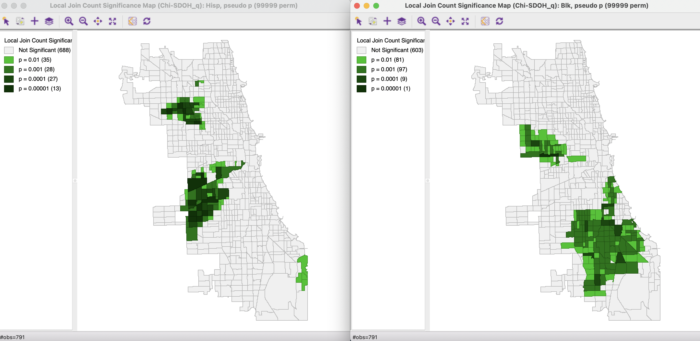
Figure 19.2: Local Join Count Significance Map
All the usual options for a significance map are available (see Chapter 16).
19.2.1.2 Saving the results
The Save Results option saves the statistic, i.e., the number of BB joins (default variable name JC), the total number of neighbors (NN), and the pseudo p-value (PP_VAL). These values are only included for those observations where \(x_i = 1\). They can be used to more closely assess the structure of specific clusters.
In practice, this can easily be detected when the results show locations with 1 like neighbor to be significant, and locations with more like neighbors not to be significant.↩︎
Note that in the original data set, the binary variables HISP50PCT and BLCK50PCT are not computed correctly. In fact, it turns out these variables are computed in the data set using a 49% cut-off percentage, which does not preclude co-location. The variables Blk and Hisp use the correct cut-off, so that co-location (majority population is more than one ethnic group) is precluded by construction.↩︎