4.5 Map Options

Once a map is created, there are three types of options available. One set pertains directly to the manipulation within the current map window, such as zooming, panning and selecting. This is implemented by means of the icons on the map toolbar (see Figure 4.10 and Section 4.5.2). The second set of options is triggered by right clicking on the map window itself. This invokes the options dialog shown in Figure 4.8, some aspects of which were already encountered in Chapter 3.

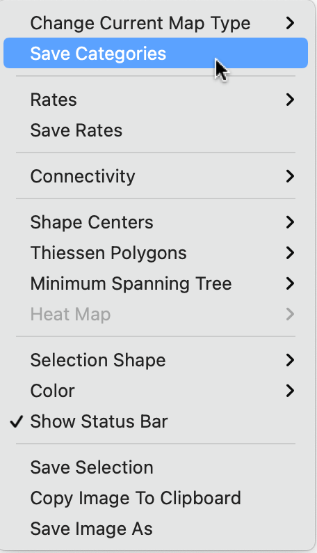
Figure 4.8: Map options

The top item (Change Current Map Type) brings up the same list with map types as invoked by clicking on the Map icon on the main toolbar (see the list in Figure 4.2). Selecting a different map type from a current map window precludes the need to choose a variable, but it also overwrites the current map.

The various features are considered in further detail below, except for the rates functions (Rates and Save Rates), and operations related to the spatial weights (Connectivity), which are covered respectively in Chapters 6 and 10. Also, the options in the fourth group (Shape Centers, etc.), were introduced earlier in Section 3.3.²⁶

A final type of customization pertains to the map legend.

4.5.1 The map legend

The map legend color shades are generated automatically from a Color Brewer palette. However, they are also fully customizable, although this is generally not recommended.

A right click on one of the legend rectangles brings up the list of options shown in Figure 4.9.²⁷ Each of the items in the list allows for the customization of an aspect, i.e., Fill Color, Outline Color, Display Precision, Scientific Notation and Background Color using the standard interfaces specific to each operating system (color wheels, as well as ways to set an explicit RGB, or CMYK value). In addition, the Copy Legend to Clipboard option makes it possible to then paste an image of the legend into any other document.

However, it should be pointed out that for most applications, the shades suggested by Color Brewer should not be changed.

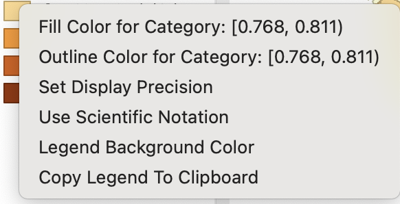
Figure 4.9: Legend Options

4.5.2 The map toolbar

The map toolbar contains ten icons that facilitate selection and viewing of the map, shown in Figure 4.10.

Figure 4.10: Map toolbar

From left to right, the icons allow the following actions:

• Select, to select one or more (using shift click) observations, or an observation region by means of a selection shape (the default is a rectangle, see Section 2.5.4); this is the default operation and works in the same fashion as selection on any graph in GeoDa

• Invert Select, switches to the complement of the current selection (same functionality as Table > Invert Selection, see Section 2.5.1.2)

• Add Map Layer, add another layer to the current map window, discussed in Section 3.6.1

• Map Layer Settings, multiple map layer interface (see Section 3.6.1)

• Zoom In, zooms in on the map by drawing a rectangle for the new map extent

• Zoom Out, zooms out of the map by repeatedly clicking on the map

• Pan, implements panning by dragging the map in any given direction with the pointer

• Full Extent, returns the map to its default full extent

• Base Map, allows the map to be superimposed onto a base layer that contains roads and other realistic geographic features (see Section 4.5.3)

• Refresh the image (in case something went wrong)

These functions are mostly standard and self-explanatory, except for the base map, which is introduced next.

4.5.3 Map base layer (base map)

The choropleth maps created by GeoDa are abstractions and lack context. To provide a way to connect the spatial distribution of a variable to the underlying reality on the ground, a base layer can be added. This shows geographical features such as roads, rivers and lakes, as well as names of places. The base layer uses the map tile concept, essentially a collection of scalable background images (it is referred to as a base map, although it is actually a picture). There are now several sources of such base layers available on the internet. GeoDa supports a limited number of these tile layer sources.

In order to add a base layer to the current map window, an active internet connection must be available (without internet, it does not work). The Base Map icon is the second from the right in the map toolbar (Figure 4.10). This brings up a list of options, shown in Figure 4.11. The default setting is No Basemap.

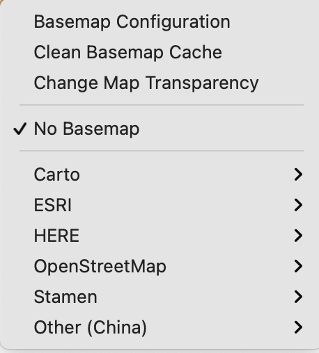
Figure 4.11: Map base layer options

Currently, GeoDa supports six main sources for base layers: Carto, ESRI, HERE, OpenStreetMap, Stamen and Other (China).²⁸ Each of these has several sub-options, which can also be customized (see Section 4.5.3.1).

For example, continuing with the Natural Breaks map for the housing variable (Figure 4.7), a base map that uses the Stamen > TonerLite option (second from bottom in Figure 4.11) with the default map transparency would provide the background illustrated in Figure 4.12. This adds the names of several places as well as some major roads (and the ocean) as the geographical context for the thematic map.

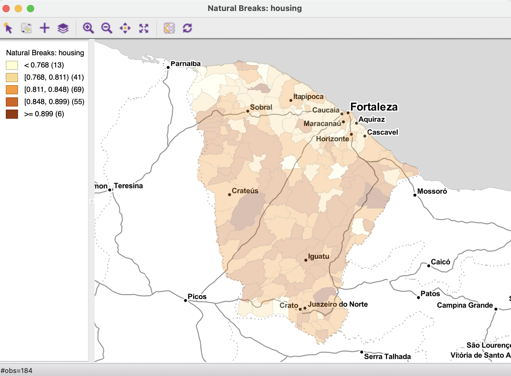
Figure 4.12: Stamen TonerLight base map, default map transparency

However, the default map transparency of 0.69 does not do justice to the features of the thematic map. The Change Map Transparency option (third item in the list in Figure 4.11) provides a slider bar to change the transparency between 1.0 (only the base layer visible) and 0.0 (only the thematic map visible).²⁹

To illustrate this effect, Figure 4.13 shows the same base layer with the transparency set to 0.40. The features of the thematic map are clearly more visible. In practice, some trial and error may be needed to find a configuration that finds the proper compromise between the thematic map and the background layer.

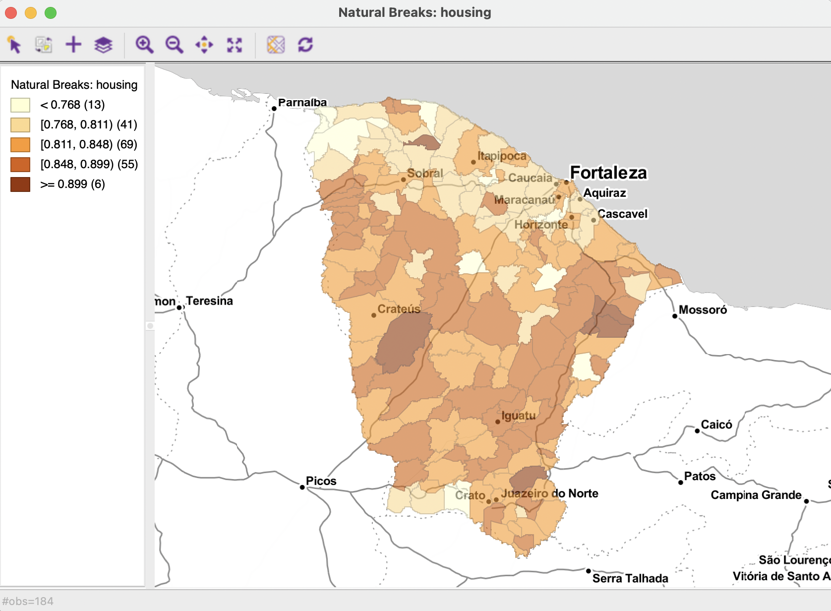
Figure 4.13: Stamen TonerLight base map, 0.40 map transparency

The various base layer sources have quite distinct design features and focus on different aspects of the geography: some have more detailed street information, others include natural features. For example, Figure 4.14 shows a base layer from the ESRI > WorldStreetMap option (with transparency set to 0.40). This provides a visual impression that is quite distinct from that in the previous maps.

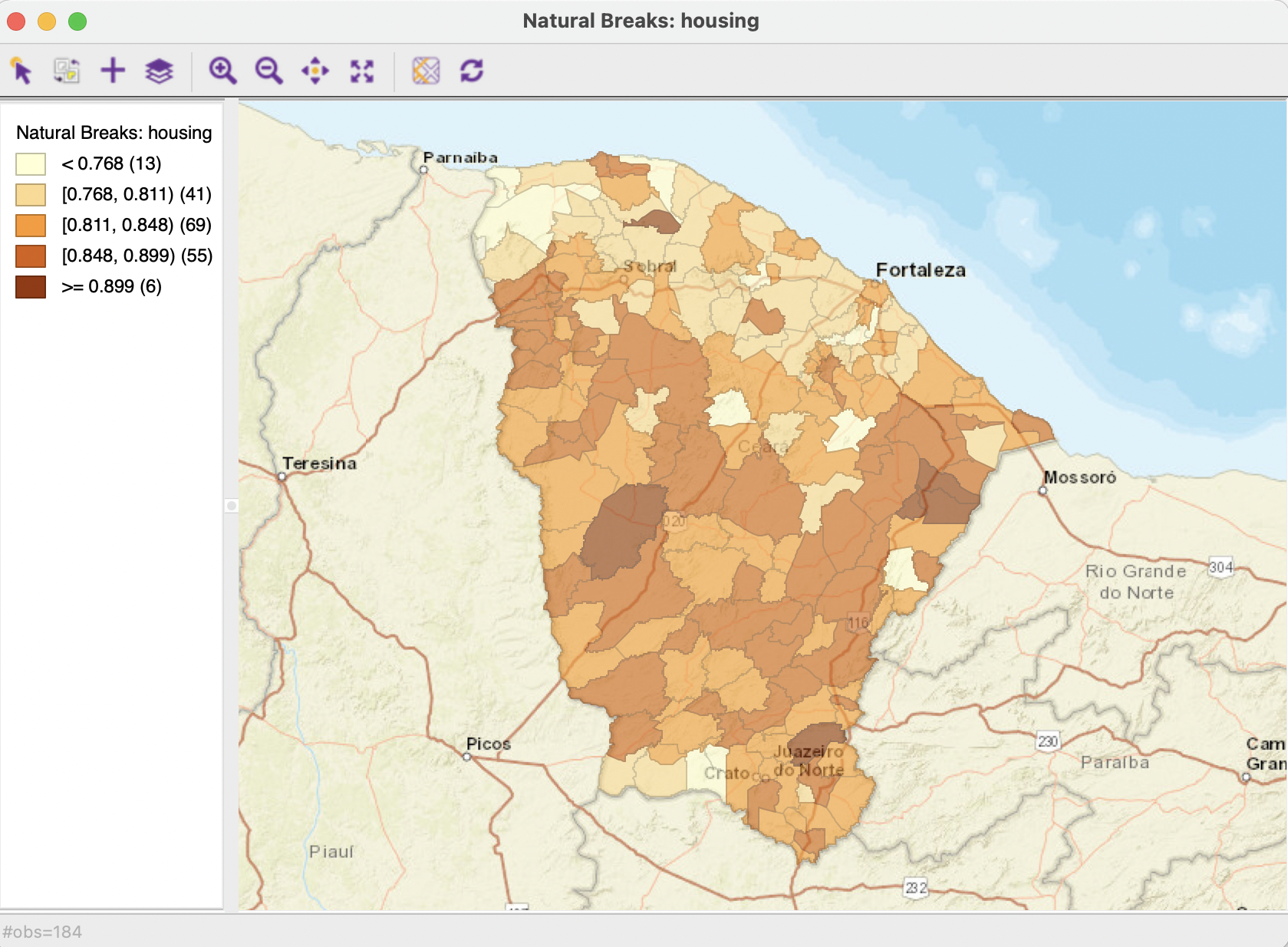
Figure 4.14: ESRI WorldStreetMap base map, 0.40 map transparency

4.5.3.1 Detailed base layer options

Each of the six base layer sources has several sub-options. These are:

• Carto: Light, Dark, Light (No Label), Dark (No Label)
• ESRI: WorldStreetMap, WorldTopoMap, WorldTerrain, Ocean
• HERE: Day, Night, Hybrid, Satellite³⁰
• OpenStreetMap: MapNik
• Stamen: Toner, TonerLite, WaterColor
• Other (China): GaoDe, GaoDe (Satellite)

The Basemap Configuration option (at the top of Figure 4.11) provides a way to further customize the sources for the base layer map tiles. Each entry corresponds with an entry in the layer options following a format group_name.basemap_name,basemap_url.³¹ In a typical application, these entries should not be touched. On the other hand, experts are free to customize.

Finally, in a pinch, it may be necessary to use the Clean Basemap Cache option when things go wrong (the second option in 4.11).

4.5.4 Saving the classification as a categorical variable

The classification associated with a given map can be added to the data table as a new categorical variable by means of the Save Categories option (the second option in Figure 4.8 ). This brings up a variable selection dialog in which the name for the new variable can be specified (the default is CATEGORIES).

Upon selecting OK, a new field is added to the data table. The categories are labeled from low to high, starting with the value 1. In the example that uses natural breaks for the housing variable (Figure 4.7), the range would go from 1 to 5. The resulting categorical variable can be used as input into a Unique Values Map or a Co-location Map (see Sections 5.3.1 and 5.3.2).

Note that there is no metadata associated with this new variable. As a result, all information is lost regarding important properties, such as the variable on which the classification is based, the type of classification, and the ranges associated with each category. To some extent, in practice, one can compensate for this lack of metadata by creative naming of variables, although this is limited by the 10 character constraint.

4.5.5 Saving the map as an image

Some other options to save features of the map are provided by the bottom three items in the menu shown in Figure 4.8. Save Selection creates an indicator variable for the selected observations, as covered in Section 2.5.4.3. For example, this allows one to create a separate indicator variables for each category in the map classification, which is often useful for later statistical analyses.³²

Copy Image to Clipboard is straightforward and allows for the image to be pasted directly into other documents.

The Save Image As option is the closest GeoDa comes to publication quality output. It allows for limited manipulation of the map view to then be saved in a standard image output format: png (the default), bmp, or SVG. For example, in Figure 4.15, the legend in the natural breaks map of Figure 4.7 was moved from the top left to the lower right corner. Limited customization is possible, such as moving and resizing legend box, changing its transparency, or even removing it altogether. Also, the image dimensions can be set precisely and the resolution specified (in dpi - the default is 300).

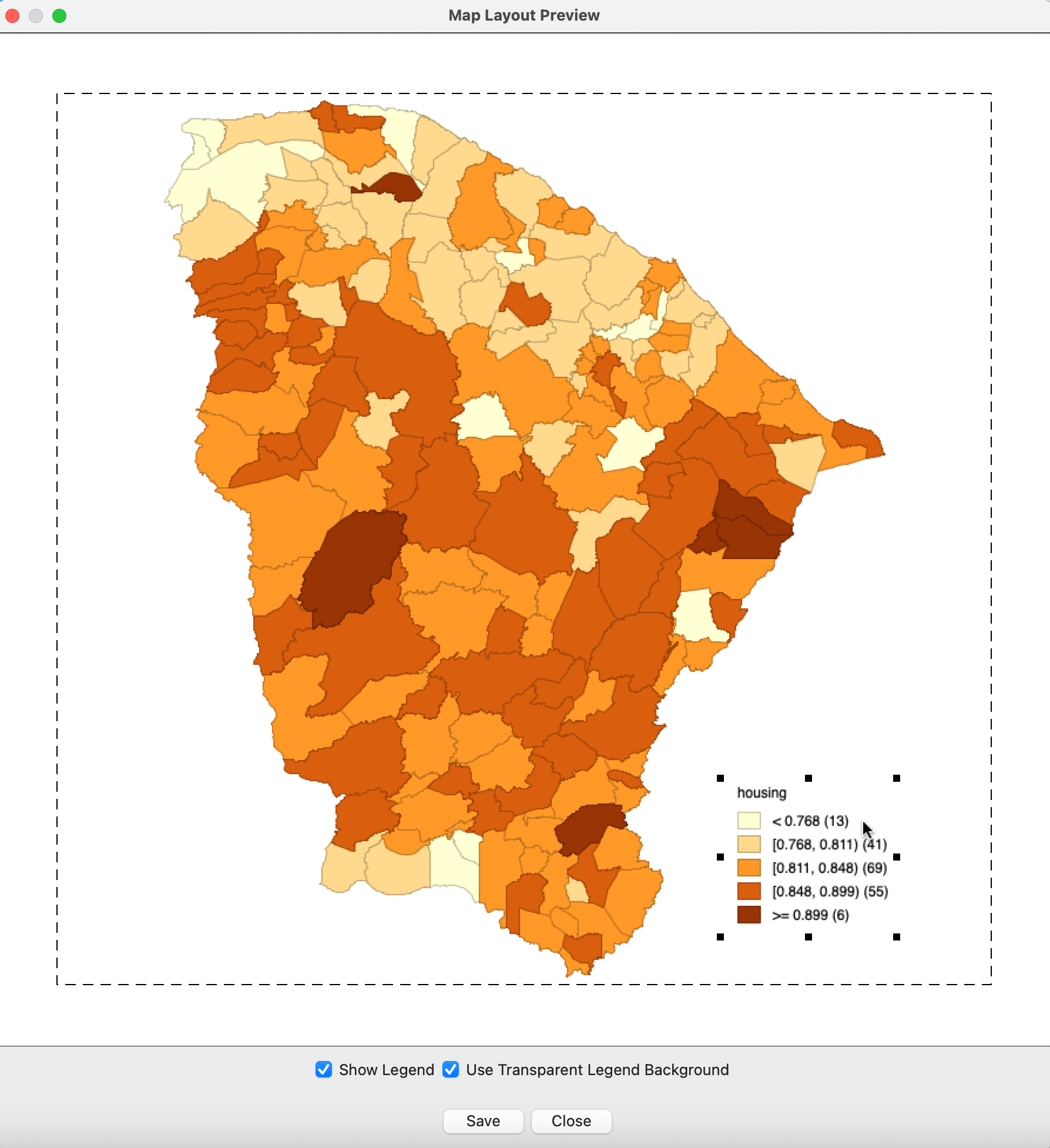
Figure 4.15: Saved Image As dialog

The saved image file can be further manipulated in specialized graphics software.

4.5.6 Other map options

The remaining three options in the Figure 4.8 menu pertain to the look of the map view. Show Status Bar is on by default, which means that the number of observations and the size of any selection will be displayed on the status bar. The Selection Shape is set by default to Rectangle, with the other two options as Circle and Line (see Section 2.5.4.1).

Finally, the Color options determine how the map is displayed. By default, the polygon outlines (i.e., in our example, the boundaries of the municipios in Ceará) are shown, with Outlines Visible checked,

By unchecking this option, the outlines disappear. This is particularly useful when the map contains many small areas that will tend to be dominated by their boundary lines. In the example in Figure 4.16, this results in an impression of larger regions compared to Figure 4.7, because many adjoining municipios end up in the same category according to the natural breaks classification.

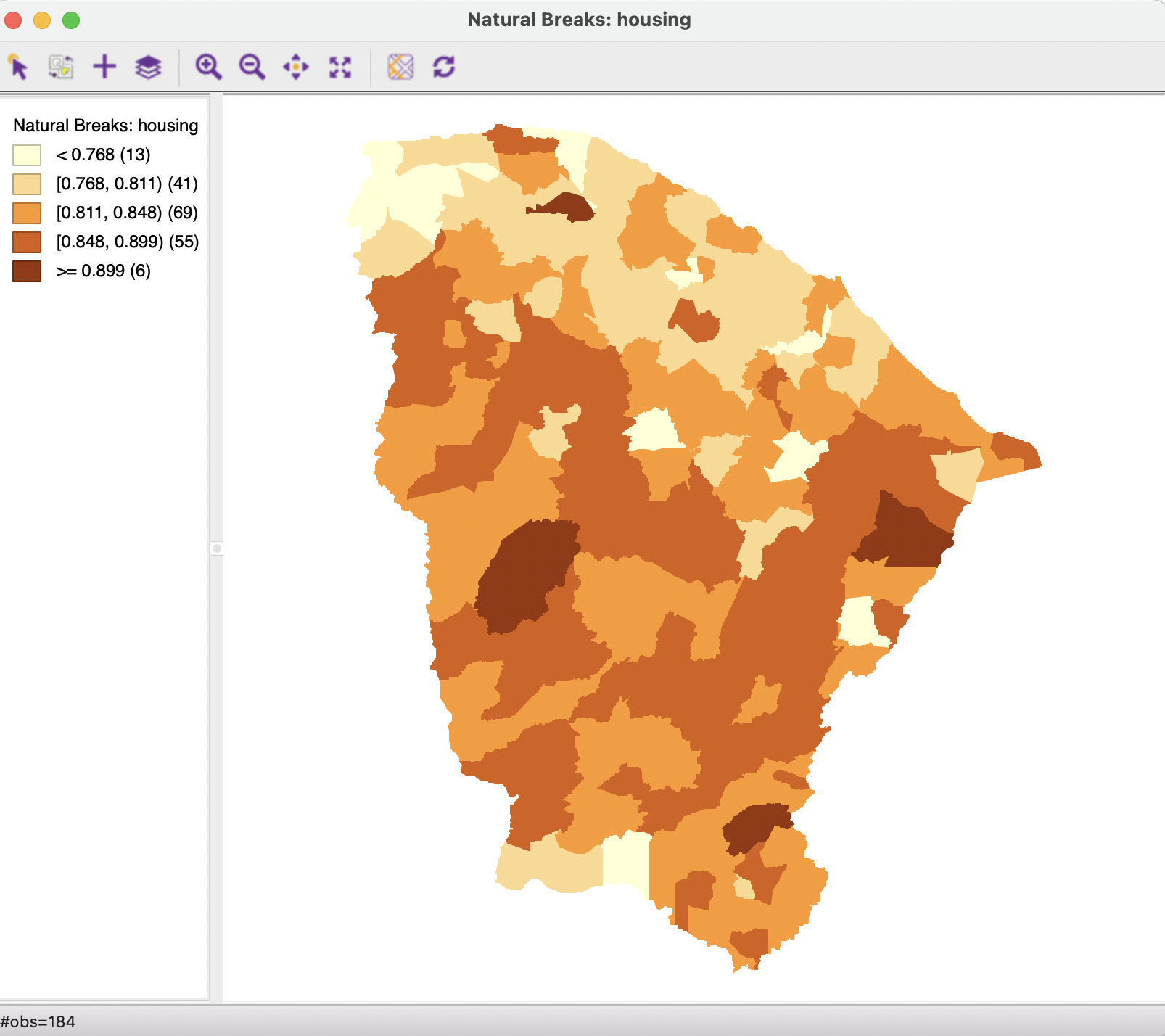
Figure 4.16: Map without outlines visible

One further option is to Show Map Boundary, only available with Outlines Visible turned off. This option is particularly useful when only a few polygons are colored in a map with many observations, for example, in the local cluster maps (Chapters 16 to 19). Turning off the outlines in such an instance makes the polygons floating in white space. With the Show Map Boundary option turned on, the initial outline of the overall map is retained.

The Background Color determines the background against which the map is drawn. In most instances, the default of white is the best choice.

---

26. The Heat Map option is covered in Chapter 20.↩︎

27. A single click selects the observations that belong to that category.↩︎

28. Other (China) contains tile data primarily aimed at users in China.↩︎

29. Note that the transparency pertains to the base layer, not to the thematic map, hence for a larger value, less of the thematic map will be visible.↩︎

30. The HERE base map support is provided under a generic account for all GeoDa users. This account has general usage restrictions, so users may want to set up their own accounts for the HERE platform. This can be accomplished by means of the Basemap Configuration option. A free HERE account can be obtained from https://developer.here.com. The basemap can then be configured with the App ID and App Key.↩︎

31. For example, the entry for Stamen > TonerLite is: Stamen.TonerLite,https://stamen-tiles-{s}.a.ssl.fastly.net/toner-lite/{z}/{x}/{y}@2x.png.↩︎

32. Select the category by clicking on its legend rectangle.↩︎