18.4 Multivariate Local Geary
In Anselin (2019a), a multivariate extension of the Local Geary statistic is proposed. This statistic measures the extent to which neighbors in multi-attribute space (i.e., data points that are close together in the multidimensional variable space) are also neighbors in geographical space. While the mathematical formalism is easily extended to many variables, in practice one quickly runs into the curse of dimensionality.
In essence, the Multivariate Local Geary statistic measures the extent to which the average distance in attribute space between the values at a location and the values at its geographic neighboring locations are smaller or larger than what they would be under spatial randomness. The former case corresponds to positive spatial autocorrelation, the latter to negative spatial autocorrelation.
An important aspect of the multivariate statistic is that it is not simply the superposition of univariate statistics. In other words, even though a location may be identified as a cluster using the univariate Local Geary for each of the variables separately, this does not mean that it is also a multivariate cluster, and vice versa. The univariate statistics deal with distances in attribute space projected onto a single dimension, whereas the multivariate statistics are based on distances in a higher dimensional space. The multivariate statistic thus provides an additional perspective to measuring the tension between attribute similarity and locational similarity.
The Multivariate Local Geary statistic is formally the sum of individual Local Geary statistics for each of the variables under consideration. For example, with \(k\) variables, indexed by \(h\), the corresponding expression is: \[c_i^M = \sum_{h=1}^k \sum_j w_{ij} (x_{hi} - x_{hj})^2.\] This measure corresponds to a weighted average of the squared distances in multidimensional attribute space between the values observed at a given geographic location \(i\) and those at its geographic neighbors \(j \in N_i\) (with \(N_i\) as the neighborhood set of \(i\)).
To achieve comparable values for the statistics, one can correct for the number of variables involved, as \(c_i^M / k\). This is the approach taken in GeoDa.
Inference can again be based on a conditional permutation approach. This consists of holding the tuple of values observed at \(i\) fixed, and computing the statistic for a number of permutations of the remaining tuples over the other locations. Note that because the full tuple is being used in the permutation, the internal correlation of the variables is controlled for, and only the spatial component gets altered.
The permutation results in an empirical reference distribution that represents a computational approach at obtaining the distribution of the statistic under the null. The associated pseudo p-value corresponds to the fraction of statistics in the empirical reference distribution that are equal to or more extreme than the observed statistic.
Such an approach suffers from the same problem of multiple comparisons mentioned for all the other local statistics. In addition, there is a further complication. When comparing the results for \(k\) univariate Local Geary statistics, these multiple comparisons need to be accounted for as well.
For example, for each univariate test, the target p-value of \(\alpha\) would typically be adjusted to \(\alpha / k\) (with \(k\) variables, each with a univariate test), as a Bonferroni bound. Since the multivariate statistic is in essence a sum of the statistics for the univariate cases, this would suggest a similar approach by dividing the target p-value by the number of variables (\(k\)). Alternatively, and preferable, a FDR strategy can be pursued. The extent to which this actually compensates for the two dimensions of multiple comparison (multiple variables and multiple observations) remains to be further investigated.121
Consequently, the interpretation of significance is difficult. In practice, extensive sensitivity analysis is recommended, using small p-values or an FDR strategy.
18.4.1 Implementation
The Multivariate Local Geary is invoked as the second item in third block in the drop down list associated with the Cluster Maps toolbar icon, or, from the menu, as Space > Multivariate Local Geary. The next dialog is a slightly different Multi-Variable Settings, which now allows for the selection of several variables (not limited to two). As usual, the spatial Weights need to be specified at the bottom of the dialog.
To illustrate this functionality, three variables are used from the Chicago SDOH sample data set. In addition to the same two as for the Bivariate Local Moran, the percentage children in poverty in 2014 (ChldPvt14), and a crowded housing index (EP_CROWD), the percentage without health insurance (EP_UNINSUR) is included as well. The latter has a correlation of 0.486 with child poverty and 0.632 with crowded housing. The spatial weights are again nearest neighbor, with \(k=6\) (Chi-SDOH_k6).
As before, the univariate properties of these variables are considered first, but now from the perspective of the Local Geary.
18.4.1.1 Univariate analysis of multiple variables
Figure 18.6 includes a box map for the percent uninsured on the left and a univariate Local Geary cluster map on the right (for 99,999 permutations with a 0.01 p-value cut-off). The box map contains three upper outliers, but otherwise boils down to the classification of a quartile map. The Local Geary cluster map reveals larger regions of High-High and Low-Low clusters, with very little evidence of negative spatial autocorrelation (only three spatial outliers).
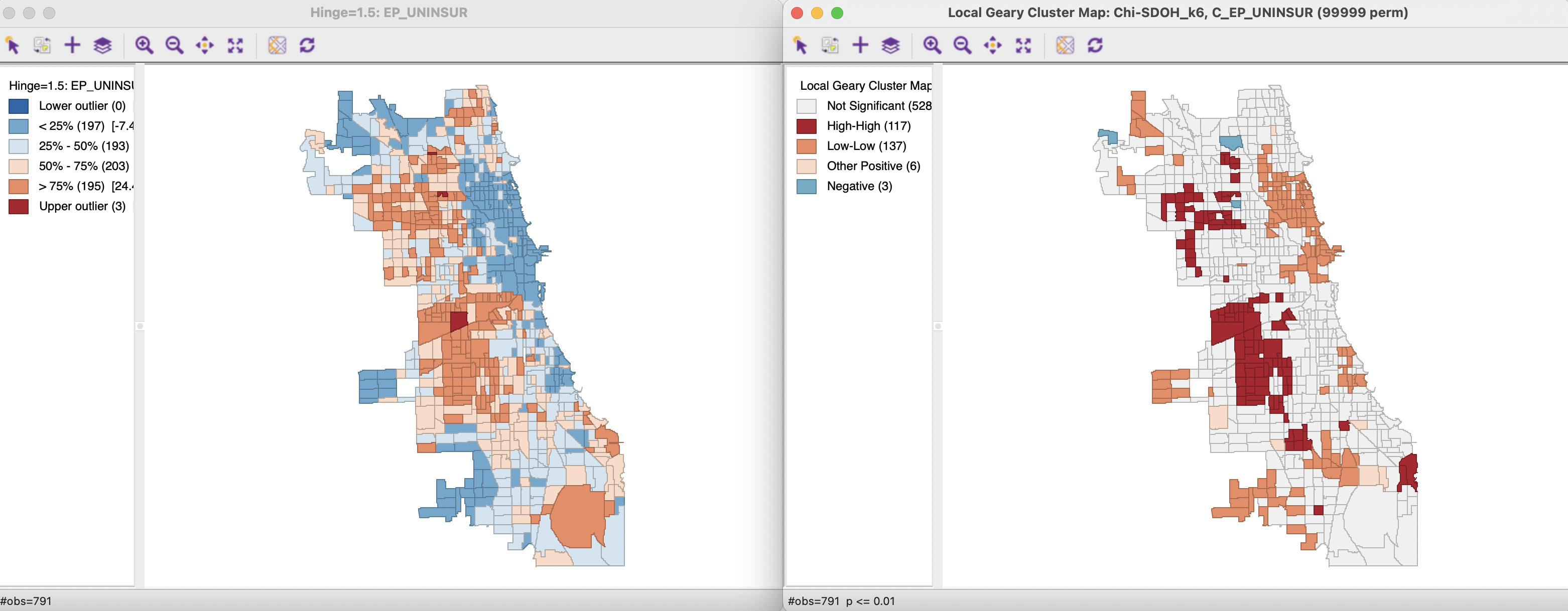
Figure 18.6: Box Map and Local Geary cluster map - Uninsured
Box maps for the other two variables were included in Figure 18.1. The corresponding cluster maps for the Local Geary (with 99,999 permutations and a p-value cut-off of 0.01) are shown in Figure 18.7. The results are similar to the broad clusters revealed for the Local Moran (Figure 18.3), but with several local differences.
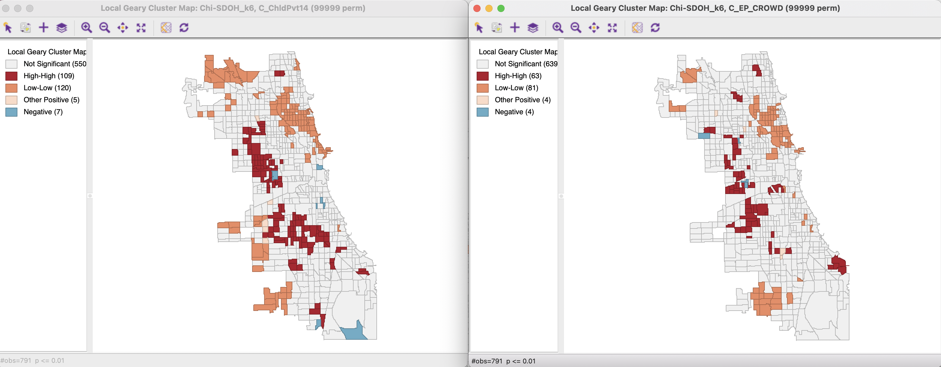
Figure 18.7: Local Geary cluster maps - Child Poverty, Crowded Housing
The commonality in local clusters between the three variables is highlighted in the co-location map in Figure 18.8. Overall, the three variables have 39 Low-Low and 10 High-High cluster cores in common, reflecting the overlap in regions of low and high values found in the univariate cluster maps.
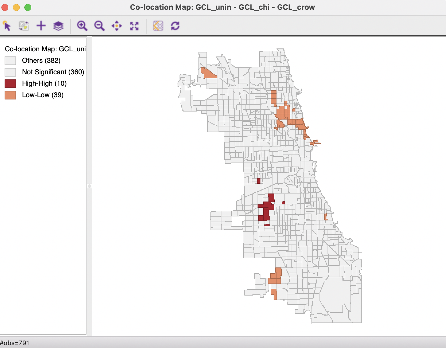
Figure 18.8: Co-Location of Local Geary
18.4.1.2 Multivariate Local Geary analysis
The significance map and cluster map for the Multivariate Local Geary, with 99,999 permutations and a p-value cut-off of 0.01 are shown in Figure 18.9. The main item that stands out is the very large number of significant observations, something surely due to the use of an inappropriate p-value cut-off. In all, 342 positive cluster cores are identified, but only two locations that suggest negative spatial autocorrelation. Even for a p-value cut-off of 0.0001, there are still 84 positive cluster cores. A careful sensitivity analysis is in order.
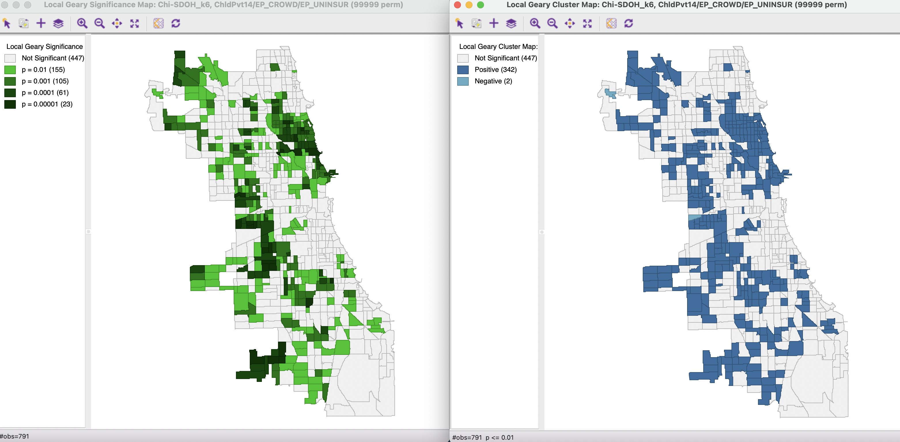
Figure 18.9: Multivariate Local Geary cluster map - Child Poverty, Crowded Housing, Uninsured
18.4.1.3 Options
All the options of the significance and cluster maps considered before remain the same. Specifically, the Save Results option offers the same choices as for the univariate Local Geary (Section 17.3.1.1).
18.4.2 Interpretation
To shed further light on where interesting locations can be found, the results for a range of different p-value cut-offs can be investigated. In Figure 18.10, the 23 observations that remain significant under the Bonferroni bound (p = 0.0000126) are linked to the univariate co-location map from Figure 18.8. Only about half (12) of these locations match between the two, pointing to other dimensions of association beyond the univariate overlap.
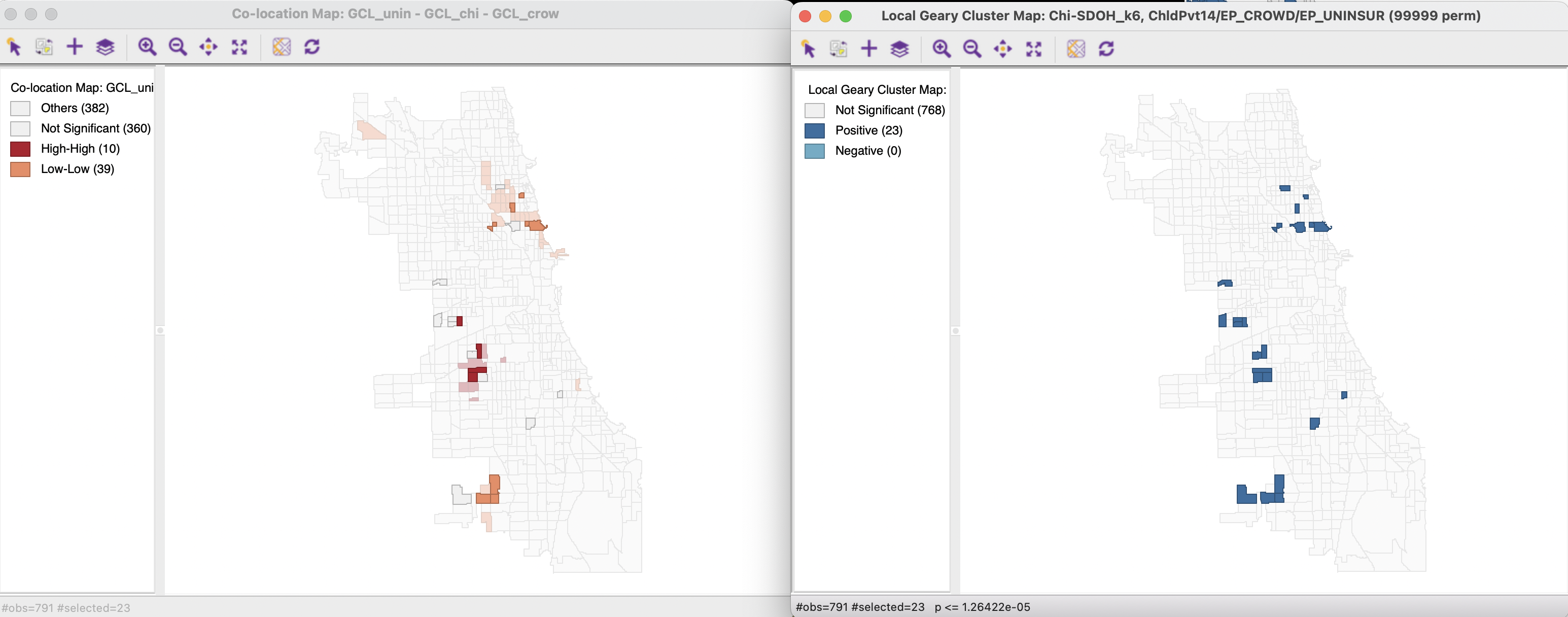
Figure 18.10: Multivariate Local Geary cluster map and Univariate Local Geary co-location
Further insight can be gained by focusing closer on those observations that are identified by the Multivariate Local Geary, but not by the univariate overlap. This then becomes much more of an exploratory exercise than a clean p-value interpretations. It should therefore be carried out with caution.
18.4.2.1 Multivariate clusters and PCP
Further insight into what the Multivariate Local Geary identifies as interesting locations can be gained from the parallel coordinate plot in the left-hand panel of Figure 18.11. The three observations in the multivariate local cluster identified using the Bonferroni bound in the right hand map are shown as three very close lines in the parallel coordinate plot. This suggests that neighbors in geographic space are also close neighbors in multi-attribute space.
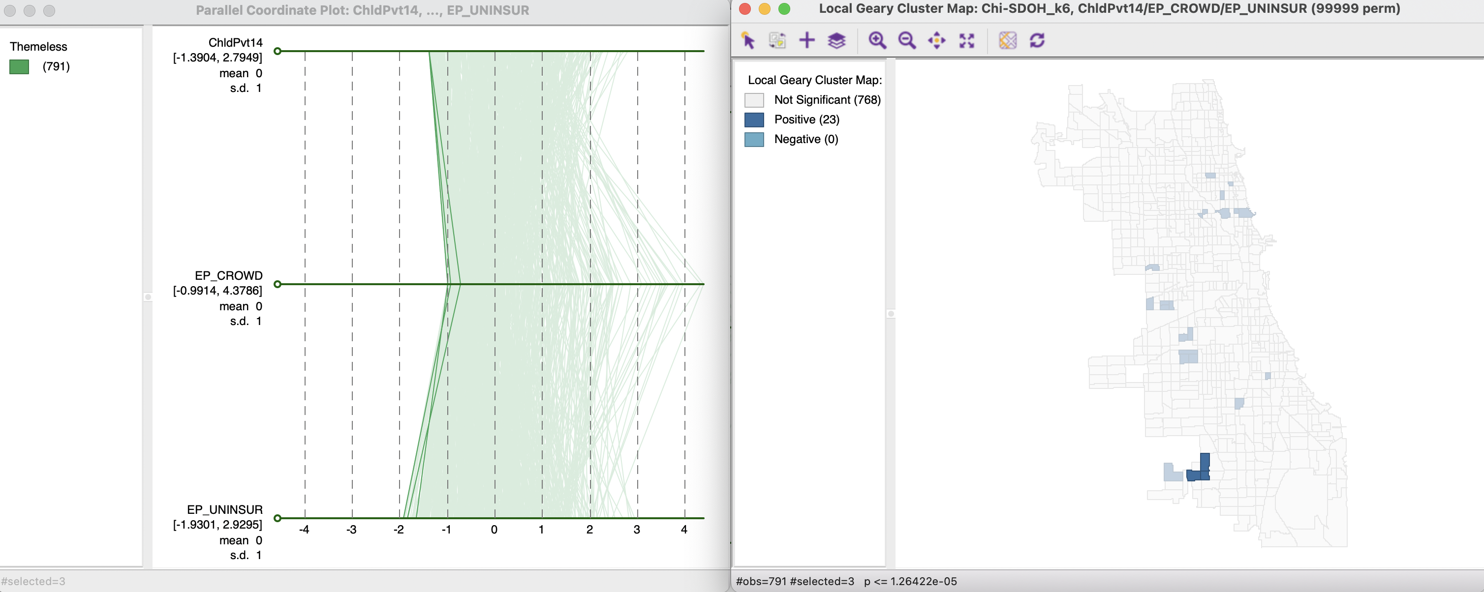
Figure 18.11: Multivariate Local Geary cluster in PCP
The connection between neighbors in geographic space and in multi-attribute space is further leveraged by the concept of a Local Neighbor Match Test, considered next.