8.2 The Curse of Dimensionality
Before considering specific techniques, it is useful to focus attention on the so-called curse of dimensionality, a concept initially conceived by Bellman (1961). In a nutshell, the curse of dimensionality means that techniques that work well in small dimensions (e.g., k-nearest neighbor searches), either break down or become too complex or computationally impractical in higher dimensions.
In the original discussion by Bellman (1961), the problem was situated in the context of optimization. To illustrate this, consider the simple example of the search for the maximum of a function in one variable dimension, as in Figure 8.2.
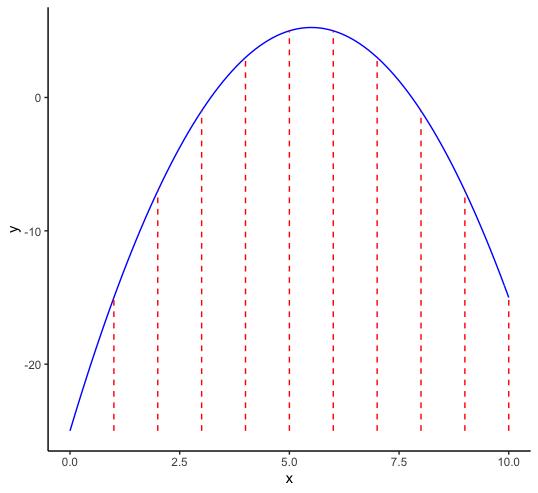
Figure 8.2: Discrete optimization in one variable dimension
One simple way to try to find the maximum is to evaluate the function at a number of discrete values for \(x\) and find the point(s) where the function value is highest. For example, in Figure 8.2, there are 10 evaluation points, equally dividing the x-range of \(0-10\). Here, the maximum is between 5 and 6. In a naive one-dimensional numerical optimization routine, the interval between 5 and 6 could then be further divided into ten more sub-intervals and so on. However, what happens if the optimization was with respect to two variables? At this stage, the attribute domain becomes two-dimensional. Using the same approach and dividing the range for each dimension into 10 discrete values now results in 100 evaluation points, as shown in Figure 8.3.
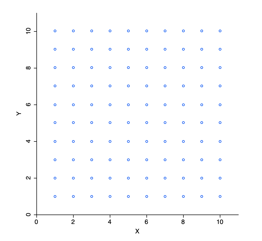
Figure 8.3: Discrete evaluation points in two variable dimensions
Similarly, for three dimensions, there would be \(10^3\) or 1,000 evaluation points, as in Figure 8.4.
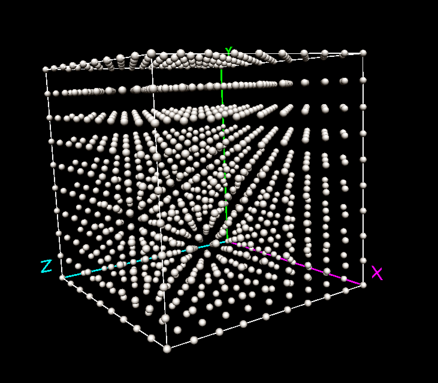
Figure 8.4: Discrete evaluation points in three variable dimensions
In general, and keeping the principle of 10 discrete values per dimension, the required number of evaluation points is \(10^k\), with \(k\) as the number of variables. This very quickly becomes unwieldy, e.g., for 10 dimensions, there would need to be \(10^{10}\), or 10 billion evaluation points, and for 20 dimensions \(10^{20}\) or 100,000,000,000,000,000,000, hence the curse of dimensionality. Some further illustrations of methods that break down or become impractical in high dimensional spaces are given in Chapter 2 of Hastie, Tibshirani, and Friedman (2009), among others.
8.2.1 The empty space phenomenon
A related and strange property of high-dimensional analysis is the so-called empty space phenomenon. In essence, the same number of data points are much farther apart in higher dimensional spaces than in lower dimensional ones. This means that in order to carry out effective analysis in high dimensions, (very) large data sets are needed.
To illustrate this point, consider three variables, say \(x\), \(y\), and \(z\), each generated as 10 uniform random variates in the unit interval (0-1). In one dimension, the observations on these variables are fairly close together, since their range will be less than one by construction.
However, when represented in two dimensions, say in the form of a scatter plot, large empty spaces appear in the unit quadrant, as in Figure 8.5 for \(x\) and \(y\) (similar graphs are obtained for the other pairs).
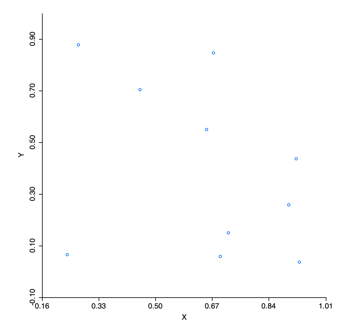
Figure 8.5: Uniform random variables in two dimensions
The sparsity of the attribute space gets even more pronounced in three dimensions, as in Figure 8.6.
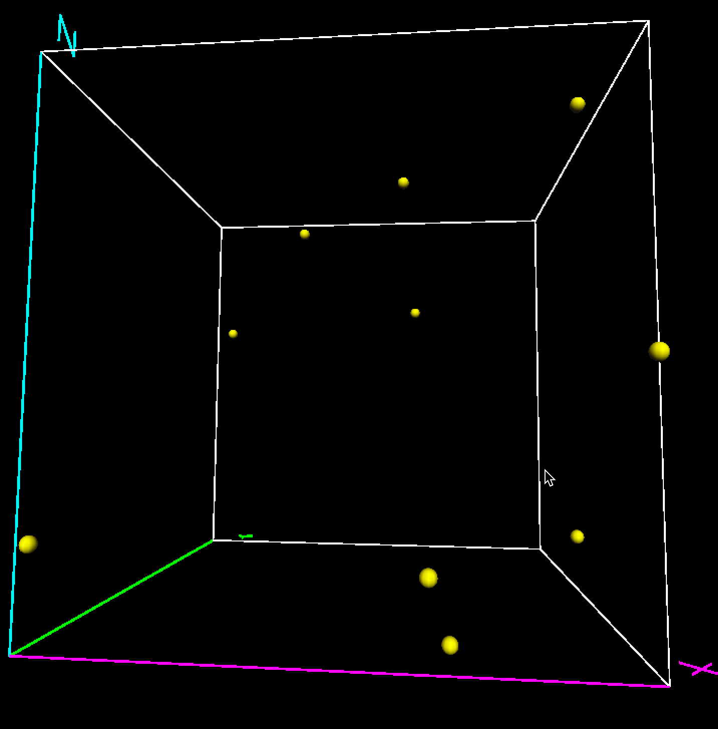
Figure 8.6: Uniform random variables in three dimensions
To quantify this phenomenon, consider the nearest neighbor distances between the observation points in each of the dimensions.56 In the example (the results will depend on the actual random numbers generated), the smallest nearest neighbor distance in the \(x\) dimension is 0.009. In two dimensions, between \(x\) and \(y\), the smallest distance is 0.094, and in three dimensions, it is 0.146. All distances are in the same units, since the observations fall within the unit interval for each variable.
Two insights follow from this small experiment. One is that the nearest neighbors in a lower dimension are not necessarily also nearest neighbors in higher dimensions. For example, in the \(x\) dimension, the shortest distance is between points 5 and 8, whereas in the \(x\)-\(y\) space, it is between 1 and 4. The other property is that the nearest neighbor distance increases with the dimensionality. In other words, more of the attribute space needs to be searched before neighbors are found. This becomes a critical issue for searches in high dimensions, where most lower-dimensional techniques (such as k-nearest neighbors) become impractical.
Further examples of some strange aspects of data in higher dimensional spaces can be found in Chapter 1 of J. A. Lee and Verleysen (2007).