18.3 Bivariate Local Moran
The treatment of the Bivariate Local Moran’s I closely follows that of its global counterpart (see Section 14.3.1). In essence, as outlined in more detail in Anselin, Syabri, and Smirnov (2002), it is intended to capture the relationship between the value for one variable at location \(i\), \(x_i\), and the average of the neighboring values for another variable, i.e., its spatial lag \(\sum_j w_{ij} y_j\). Apart from a constant scaling factor (that can be ignored), the statistic is the product of \(x_i\) with the spatial lag of \(y_i\) (i.e., \(\sum_j w_{ij}y_j\)). In order to make this operational and easier to interpret, both variables should be standardized, such that their means are zero and variances equal one. The Bivariate Local Moran is then:
\[ I_{i}^B = x_i \sum_j w_{ij} y_j,\] in the usual notation.
As is the case for its global counterpart, this statistic needs to be interpreted with caution, since it ignores the correlation between \(x_i\) and \(y_i\) at location \(i\) (see also Section 14.3.1).
A special case of the Bivariate Local Moran statistic is when the same variable is compared in neighboring locations at different points in time. The most meaningful application is where one variable is for time period \(t\), \(z_t\), and the other variable is for the neighbors in the previous time period, \(\sum_j w_{ij}z_{t-1}\). This formulation measures the extent to which the value at a location in a given time period is correlated with the values at neighboring locations in a previous time period, or an inward influence. An alternative view is to consider \(z_{t-1}\) and the neighbors at the current time, \(\sum_j w_{ij}z_{t}\). This would measure the correlation between a location and its neighbors at a later time, or an outward influence. The first specification is more accepted, as it fits within a standard space-time regression framework.
Inference proceeds similar to the global case, but is now conditional upon the tuple \(x_i, y_i\) observed at location \(i\). This somewhat controls for the correlation between \(x\) and \(y\) at \(i\). The remaining values for \(y\) are randomized and the statistic is recomputed to create a reference distribution. The usual caveats regarding the interpretation of significance apply here as well.
18.3.1 Implementation
The Bivariate Local Moran I is invoked as the third item in the drop down list associated with the Cluster Maps toolbar icon, or, from the menu, as Space > Bivariate Local Moran’s I. The next dialog is the customary Variable Settings, which now has two columns, one for First Variable (X), and one for Second Variable (Y). Since the Bivariate Local Moran is not symmetric, the order in which the variables are specified matters. At the bottom of the dialog, the Weights need to be selected.
To illustrate this feature, two variables are used from the Chicago SDOH sample data set: the percentage children in poverty in 2014 (ChldPvt14), and a crowded housing index (EP_CROWD). The spatial weights are nearest neighbor, with \(k=6\) (Chi-SDOH_k6).
Before proceeding with the actual bivariate analysis, the univariate characteristics of the spatial distribution of each variable are considered more closely.
18.3.1.1 Univariate description of two variables
Figure 18.1 shows a box map for each of the variables. On the left, for ChldPvt14, there are no outliers, so the box map corresponds with a simple quartile map. In contrast, the map for EP_CROWD has 27 upper outliers, somewhat scattered around the city.
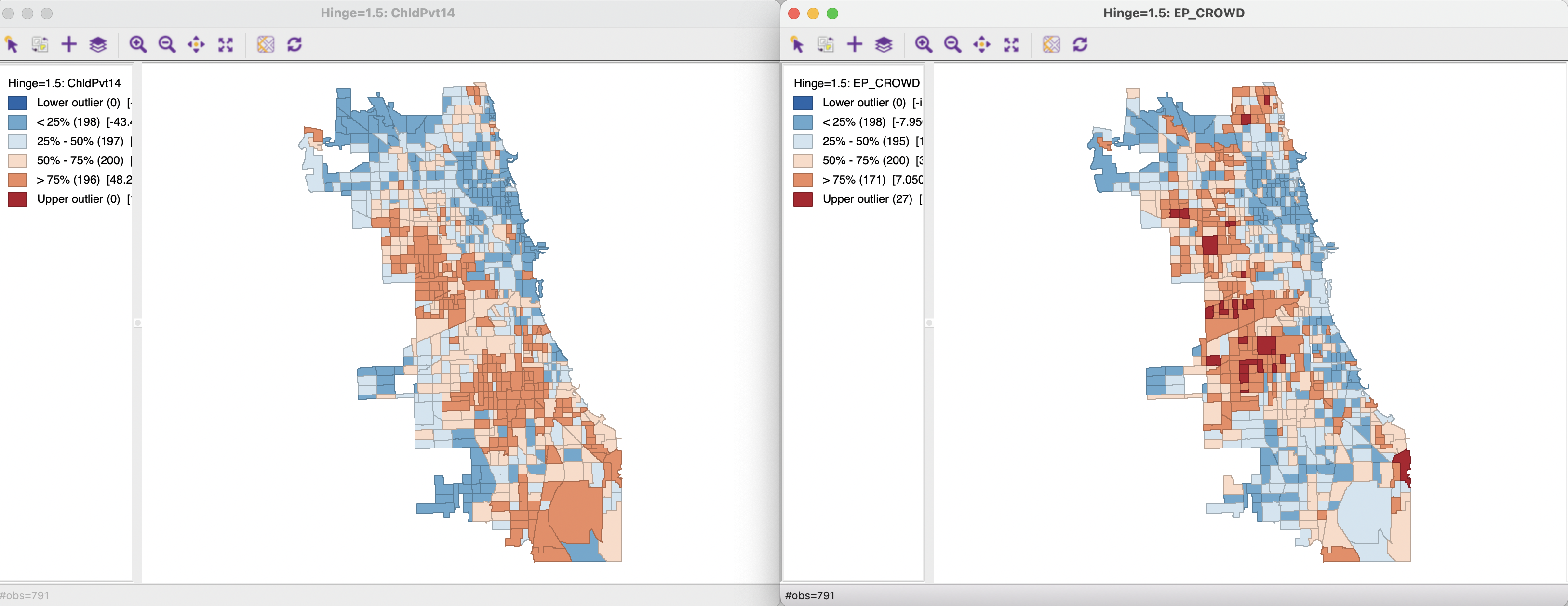
Figure 18.1: Box maps - Child Poverty and Crowded Housing
The correspondence between the two spatial distributions is highlighted in the co-location map in Figure 18.2.119 This map shows the census tracts where the observations for both variables fall in the same quartile category. In this example, this is appropriate, since both variables work in the same direction (higher values are worse conditions). The classifications match for 284 out of 791 observations, or 36 %. The bulk of the matches is for the lowest quartile (i.e., better conditions), where 109 out of 198 observations match. About half that many locations also match for the three other categories (clearly, there are no matches for the outliers, since those are only present in one of the maps). The co-location map provides an initial sense of the degree of spatial correspondence between the two variables. More formally, the (non-spatial) correlation coefficient between the two is 0.392.
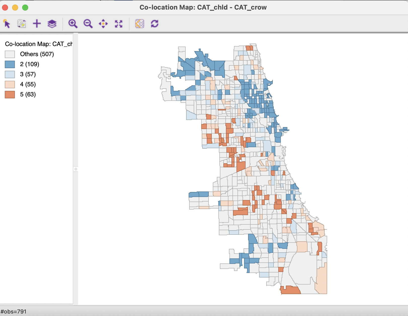
Figure 18.2: Co-Location of Child Poverty and Crowded Housing
18.3.1.2 Univariate Local Moran for each variable
To provide further context, the cluster maps for the univariate Local Moran for each variable (using 99,999 permutations with a cut-off p-value of 0.01) are shown in Figure 18.3. In both maps, the largest share consists of Low-Low cluster cores (118 for child poverty and 102 for crowded housing), but for child poverty this is almost equally balanced by High-High cores (101). For crowded housing, there are clearly much fewer High-High cores (67). In both instances, the cluster cores constitute a small number of larger regions, with very few spatial outliers.
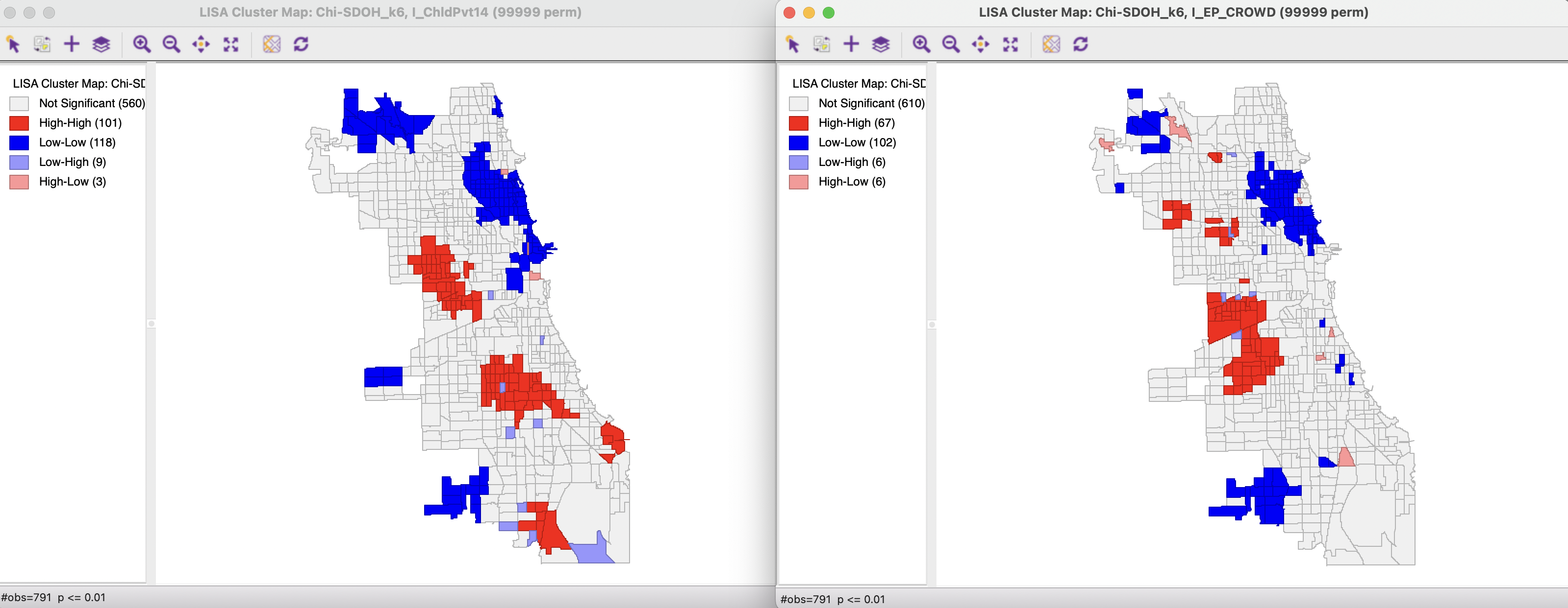
Figure 18.3: Local Moran cluster map - Child Poverty and Crowded Housing
The correspondence between the two cluster maps is further highlighted in Figure 18.4, which shows a co-location map for the cluster classifications.120 Almost 3/4 of the Low-Low cluster cores match between the two variables, but this is only the case for 15 High-High cores. Since a cluster consists of the core and its neighbors, the actual match has a somewhat wider reach than just the cluster cores. None of the spatial outliers occur in the same location.
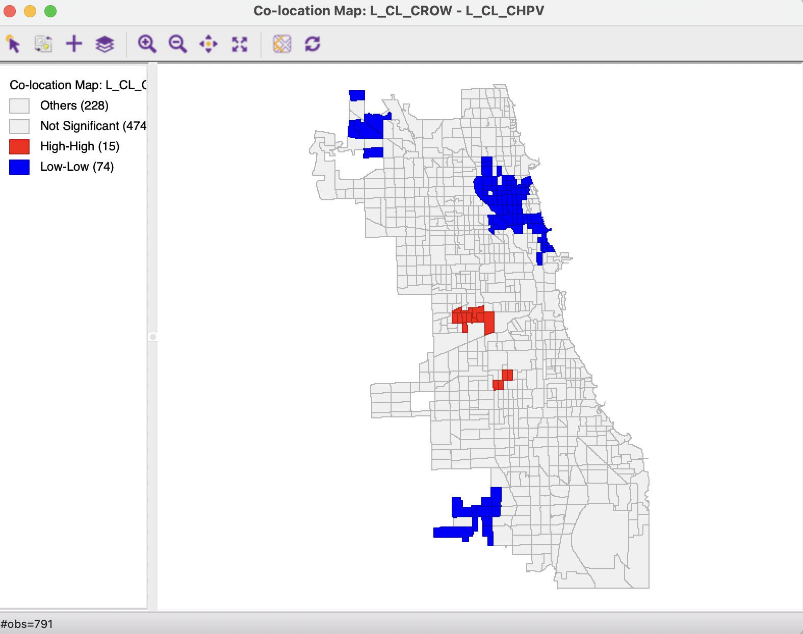
Figure 18.4: Co-Location of Local Moran for Child Poverty and Crowded Housing
18.3.1.3 Bivariate analysis
The cluster maps for the Bivariate Local Moran are shown in Figure 18.5, using 99,999 permutations and a p-value cut-off of 0.01. The map on the left is for child poverty surrounded by crowded housing, the map on the right for crowded housing surrounded by child poverty. Clearly, the cluster maps are different, in accordance with the lack of symmetry for this statistic. Both maps are characterized by many more spatial outliers than in the univariate cluster maps, highlighting locations where a high/low value for one variable is surrounded by neighbors with the opposite, i.e., low/high values.
The common cluster cores from the univariate maps (Figure 18.4) are present in both bivariate maps. In fact, a co-location map based on the two bivariate maps yields the exact same result as Figure 18.4. This makes intuitive sense, since a bivariate High-High cluster requires a High value for one variable (cluster core) to be surrounded by High values for the other variable (neighbors part of the cluster surrounding the matching cluster core). The same holds for the Low-Low clusters.
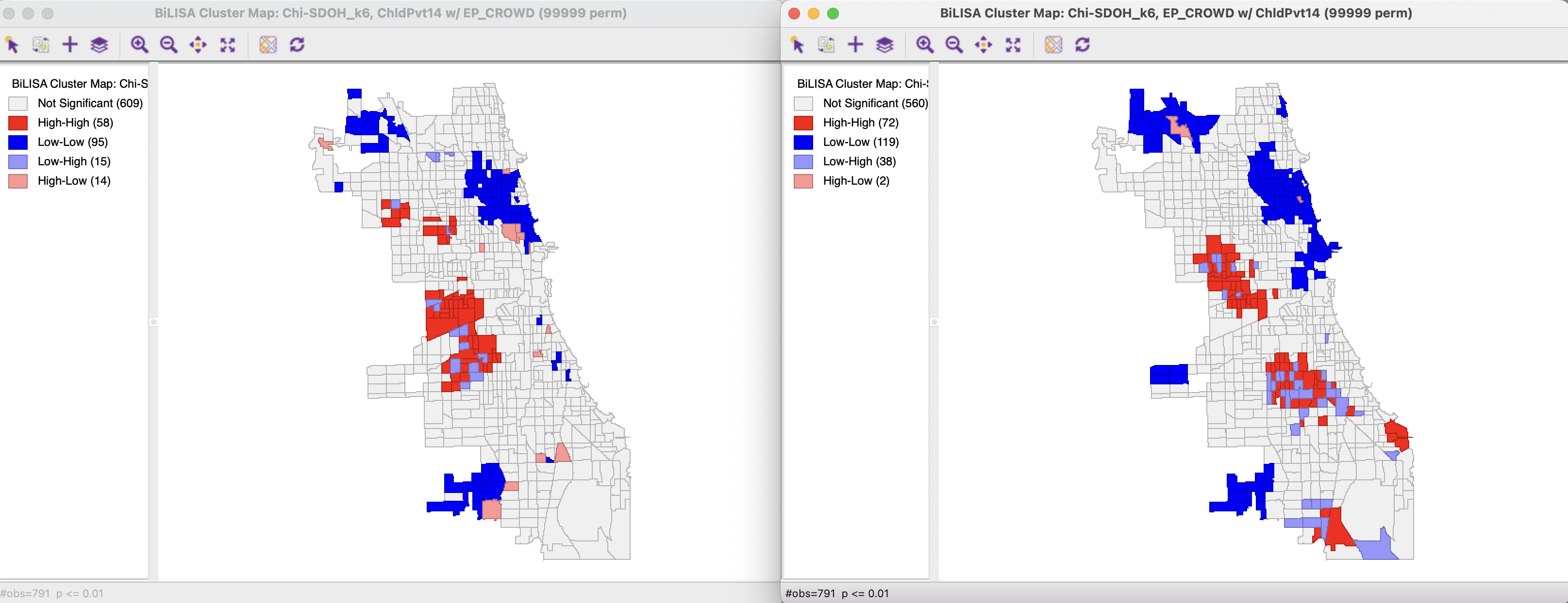
Figure 18.5: Bivariate Local Moran cluster map - Child Poverty and Crowded Housing
Arguably, the more interesting information follows from the location of the spatial outliers, especially the Low-High outliers, of which there are 15 for child poverty-crowded housing and 38 for crowded housing-child poverty. These are census tracts where a Low (good) value for one indicator is surrounded by a High (bad) value for the other, or vice versa, more so than expected under spatial randomness. This is information the univariate cluster maps cannot provide.
18.3.1.4 Options
The Bivariate Local Moran has all the same options as the conventional Local Moran, as detailed in Chapter 16. The cluster codes associated with saved results are the same as well.
18.3.2 Interpretation
The interpretation of the Bivariate Local Moran needs to be carried out very carefully. Aside from the usual caveats about multiple comparisons and p-values, the association between one variable and a different variable at neighboring locations needs to consider the in-situ correlation between the two variables as well. As the discussion in the previous sections illustrates, it is best to combine the bivariate analysis with a univariate analysis for each variable. In addition, it is important to consider both directions of association. This will tend to reveal strong local clustering among the two variables as well as instances where their spatial patterns do not coincide in the form of bivariate spatial outliers.
The map is constructed after saving the map categories for both box maps, followed by Map > Co-location Map, using the classification codes and a Box Map classification for the co-location map.↩︎
This is accomplished after saving the cluster classifications for both cluster maps, followed by Map > Co-location Map, using the cluster codes and a LISA Map classification for the co-location map.↩︎