13.2 Spatial Randomness

Spatial randomness is the point of departure in any statistical analysis of spatial pattern. It is the null hypothesis against which the data are compared.

Spatial randomness is the absence of any systematic spatial structure in the data, i.e., there are no distinct patterns. The location of a given observation is of no value as a piece of information, such that the where does not matter. In other words, the notion of spatial randomness is not very interesting other than as a statistical concept. The main goal of an analysis is to reject the null hypothesis of spatial randomness in favor of the presence of some type of pattern. This is accomplished by means of a test statistic.

Spatial randomness can be interpreted in two main ways, which correspond to different approaches towards spatial analysis. In one, representing a simultaneous view, the observed spatial pattern is viewed as equally likely as any other spatial pattern. More specifically, it is the pattern as a whole that is considered. Another view represents a conditional perspective. It implies that the value observed at a given location does not depend on the values observed at neighboring locations. Again, this requires that location does not matter. Fundamentally, the two notions are equivalent, but they result in different statistical approaches.

Before considering specific statistics (see Section 13.4), two perspectives toward making spatial randomness operational are briefly outlined. One is based on a parametric assumption, specifying observations as independent and identically distributed (i.i.d.). The other perspective does not assume a particular distribution, although it still requires identical distributions, especially a constant variance. In such an approach, the location of the observations may be altered without affecting the information content of the data. This is referred to as randomization, in the sense that each observed value has the same probability of being associated with any of the locations, i.e., the map is irrelevant.

13.2.1 Parametric approach

The parametric approach requires the assumption of a specific distribution. Typically, this is the normal (or Gaussian) distribution, since it has the important property that lack of correlation also implies independence. For other distributions, this is not the case.

The simplest implementation of spatial randomness is to take a collection of uncorrelated (independent) standard normal variates. Since nothing spatial is assumed for this distribution, the result is spatially random.

For example, Figure 13.2 illustrates the layout of 100 standard normal variates on a 10 \(\times\) 10 square grid, using a quantile map with six categories. Even though one may be tempted to see structure in the data, this would be purely coincidental, since the map is devoid of pattern by construction.

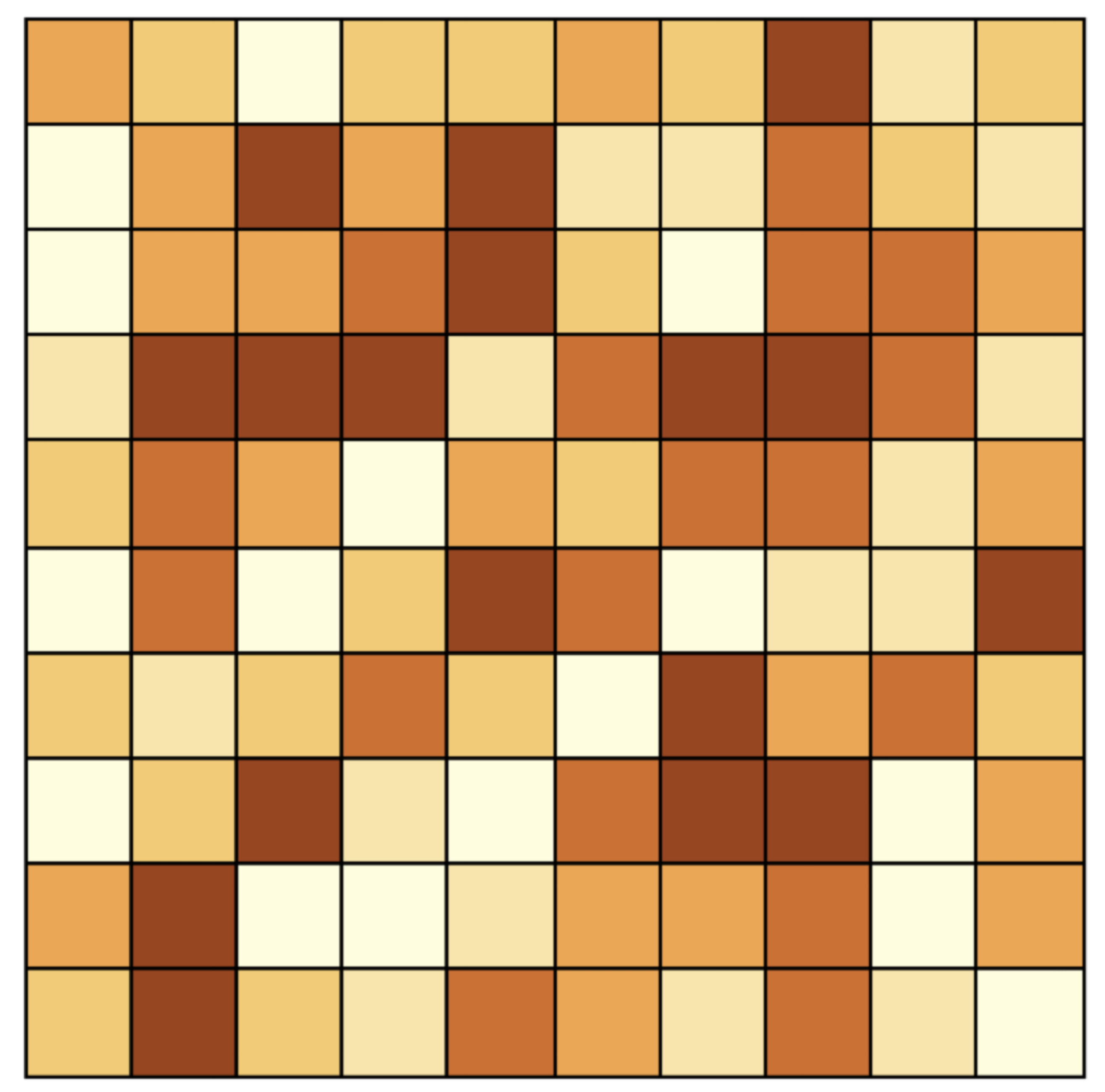
Figure 13.2: Spatially random observations - i.i.d

13.2.2 Randomization

The randomization approach does not require the selection of a specific parametric distribution for the data. Instead, it takes advantage of the property that under the null hypothesis, each observation is equally likely to be at any location. By randomly permuting or reshuffling the data across locations, the concept of spatial randomness can be simulated.

For example, the left hand panel of Figure 13.3 shows the spatial distribution of the income per capita for the 77 Chicago community areas (from the 2015-2019 ACS) as a quantile map with eight categories. On the right, the same 77 values are randomly allocated to community areas, resulting in a totally different map. The true map illustrates the well-known pattern of higher incomes in the northern part of the city, contrasting with low income in the south and west. By contrast, the randomized map shows no such pattern. High income areas (dark brown) are found all over the city, without any apparent structure to their locations.

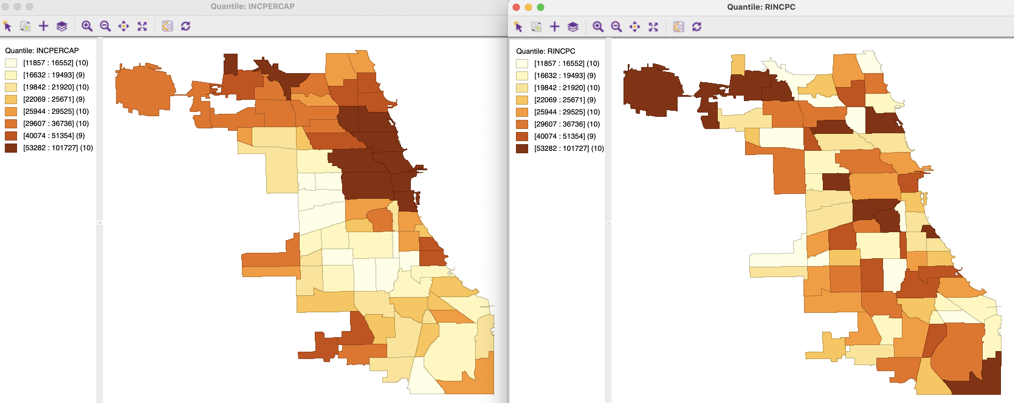
Figure 13.3: Spatially random observations - true and randomized per capita income

Parenthetically, the contrast between the two maps illustrates the value of a spatial perspective. Taken as such, the statistical distribution of the original and randomized variables are identical. In Figure 13.4, an eight category histogram highlights this property. In other words, the a-spatial perspective on the data distribution offered by the histogram for the two variables cannot account for the important distinction between their spatial patterns.

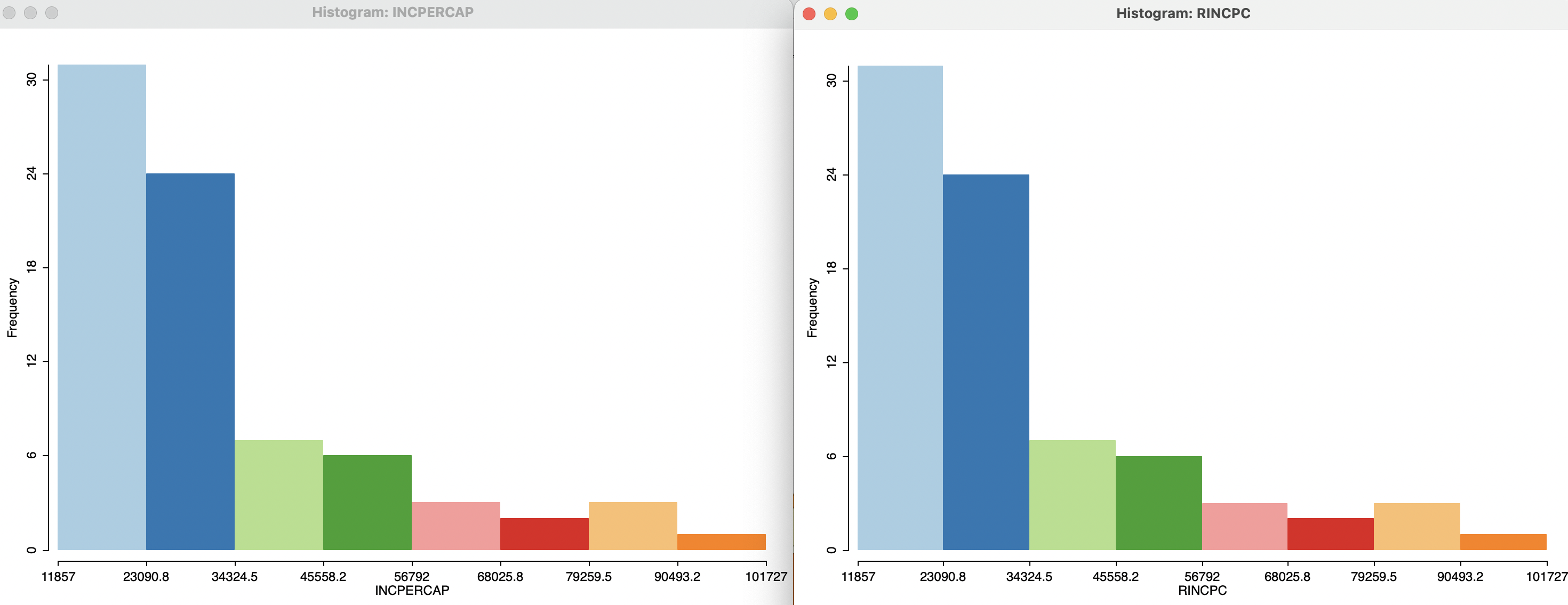
Figure 13.4: True and randomized per capita income - histograms

13.2.3 Simulating spatial randomness

The spatially randomized map in Figure 13.3 is obtained by creating a new variable, taking advantage of the Calculator functionality in the table. Specifically, as listed in Section 2.4.2.2, the Univariate operations include a Shuffle function, which implements randomization. Operationally, the list of index numbers of the observations is randomly reshuffled and the original observations are assigned to the new locations. For example, if the original list was 1, 2, 3, 4, 5, and the randomized list yields 3, 2, 4, 5, 1, then the value at location 1 will be assigned to location 3, 2 will remain in place, 3 will move to spot 4, 4 to spot 5, and 5 to location 1.

The randomization (or permutation) approach is an essential tool to create many versions of the data under the null hypothesis. This is particularly useful, since, except in highly stylized situations (e.g., standard normal distribution), it quickly becomes very difficult to obtain the properties of any spatial autocorrelation statistic by means of an analytical derivation.