3.7 Spatial Join
The multi-layer infrastructure allows for the calculation of variables for one layer, based on the observations in a different layer. This is an example of a point in polygon GIS operation. There are two applications of this process. In one, referred to as Spatial Assign, the ID variable (or any other uniquely identifying variable) of a spatial area is assigned to each point that is within the area’s boundary. The reverse of this process is Spatial Count, i.e., a count or other form of aggregation over the number of points that are within a given area, similar to the operation of Aggregation and Dissolve (see Section 3.5).
Even though the default application is simply assigning an ID or counting the number of points, more complex assignments and aggregations are possible as well. For example, rather than just counting the points, an aggregate over the points can be computed for any variable, such as the mean, median, standard deviation, or sum across the point observations for that variable.
It is important to keep in mind the order in which the layers are loaded into the multi-layer setup. For spatial assign, the point layer is first, since the areal unit identifier is assigned to each point. As mentioned before, only the table of the first loaded layer is available for manipulation or analysis. So, in order to add the ID code to the point layer table, it must be loaded first.
For spatial count, the reverse is the case. The polygon layer needs to be loaded first, since the number of points (or any other aggregation) is added to the table with observations for the areal units.
This functionality is invoked from the menu as Tools > Spatial Join, or by selecting the Spatial Join option from the Tools icon in Figure 2.1.
3.7.1 Spatial assign
To illustrate the spatial assign application, the layer arrangement from Figure 3.19 is considered, with the (projected) car jacking locations loaded first, followed by the (projected) community area boundaries.
Invoking Tools > Spatial Join generates the dialog shown in Figure 3.24. This differs slightly between the spatial assign and spatial count functionalities (see Figure 3.27 for the latter).
The dialog shows how the current map layer, Chicago_carjack_2020_pts is joined to another layer. In the example, there is only one other layer, i.e., community_areas_proj, but in general, there could be several layers to select from. The ID Variable list shows all the variables that could serve as unique identifiers for the areal units. In the example, there are three variables listed, but only the fist two pertain to the community areas in the map layer (all integer variables are listed by default). In Figure 3.24, area_num_1 is selected as the ID variable.
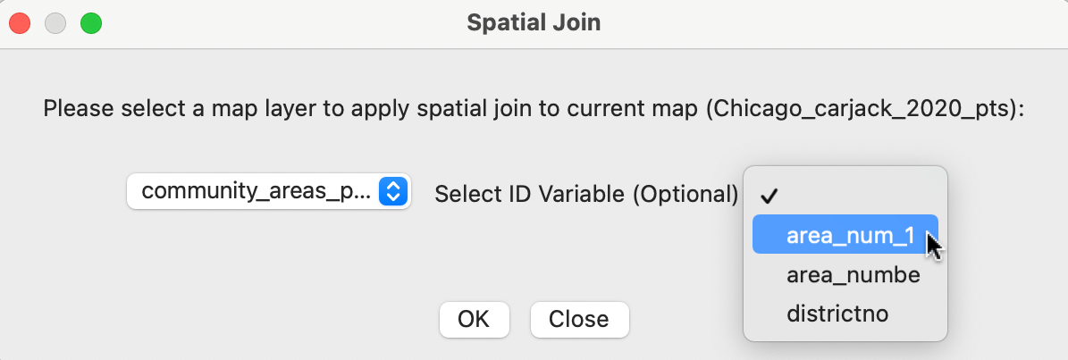
Figure 3.24: Spatial join dialog – areal unit identifier for point
The next dialog requests the variable name of the spatial assign variable, which is SA by default. After specifying the variable name, it is added to the data table for the point layer. In Figure 3.25, the new SA column is listed next to the original Commu_Area variable from the point location data base. A quick check confirms that they are the same. The difference is that the values for the SA variable were derived from a spatial point in polygon operation, joining the two layers, whereas the original variable was included during data entry.
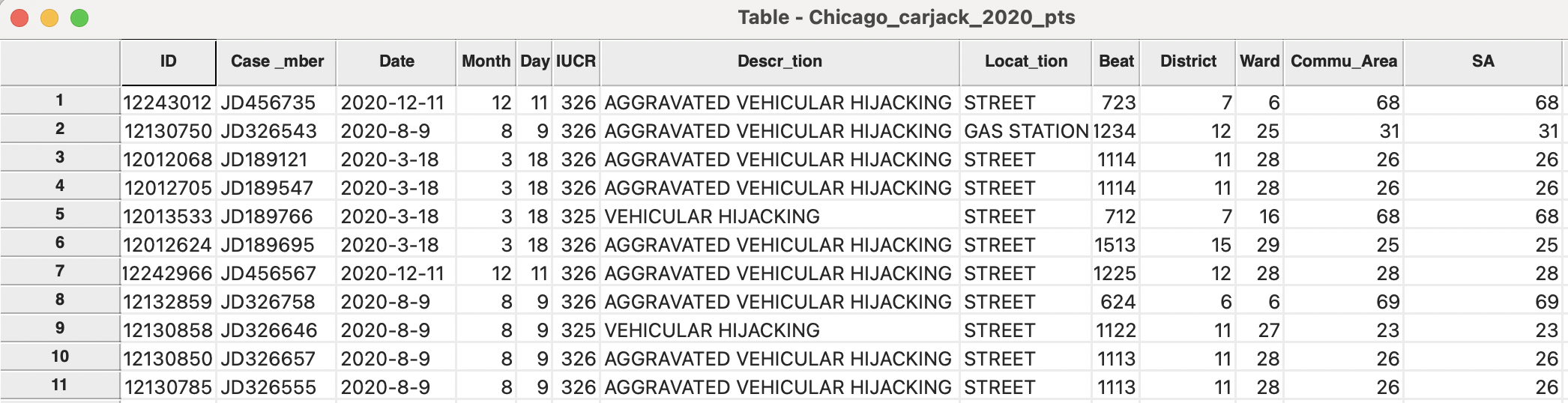
Figure 3.25: Community area identifier (SA) in point table
In cases where the point in polygon operation results in a mismatch (e.g., due to differences in precision of the location coordinates in the two layers), a value of -1 is used for the spatial assign. In the example, there are three such points, all situated at the very edge of a polygon. This is illustrated in Figure 3.26 for the two mismatches at the southern and south-western edge of the city (one other mismatch is in the very north).
Depending on the goals of the analysis, one could either eliminate the points from the data set, or manually edit the values in the table after zooming in on the actual location.
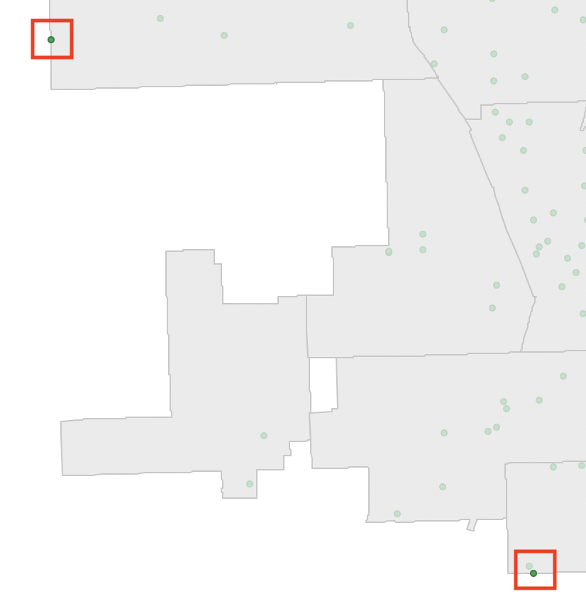
Figure 3.26: Point in polygon mismatch
The new spatial assign variable can now be used to aggregate observations, as in Section 3.5. However, the dissolve operation does not work, since there is no boundary information associated with the points. Their spatial information consists of the coordinates only, which do not lend themselves to a dissolve operation.
As always, a File > Save or File > Save As operation must be used to make the addition of the spatial assign variable permanent.
3.7.2 Spatial count
To illustrate the spatial count feature, the order of the two layers from Figure 3.19 is reversed. The community_areas_proj layer is loaded first (since the counts will be added to the polygon table observations), followed by Chicago_carjack_2020_pts. Note that in order to make the point layer visible, it needs to be moved to the top.22
The Tools > Spatial Join command generates the dialog shown in Figure 3.27. In the default setup, the Spatial Count radio button is checked, which does not require any further input. In the figure, the Spatial Join option is shown, which is essentially the same as aggregation (Section 3.5). Several variables can be selected, with the aggregation following Sum, Mean, Median or Standard Deviation.
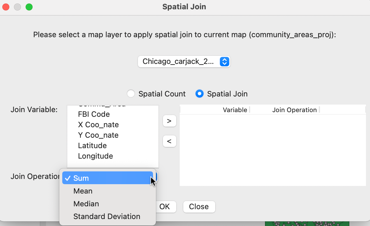
Figure 3.27: Spatial join dialog – aggregation options
In the illustration, the default is used, i.e., Spatial Count. The next dialog asks to specify the variable name for the result, with the default as SC. This yields a new variable in the table, which shows the number of car jackings occurring in each community area, as illustrated in Figure 3.28. As before, the addition only becomes permanent after a File > Save or File > Save As operation.
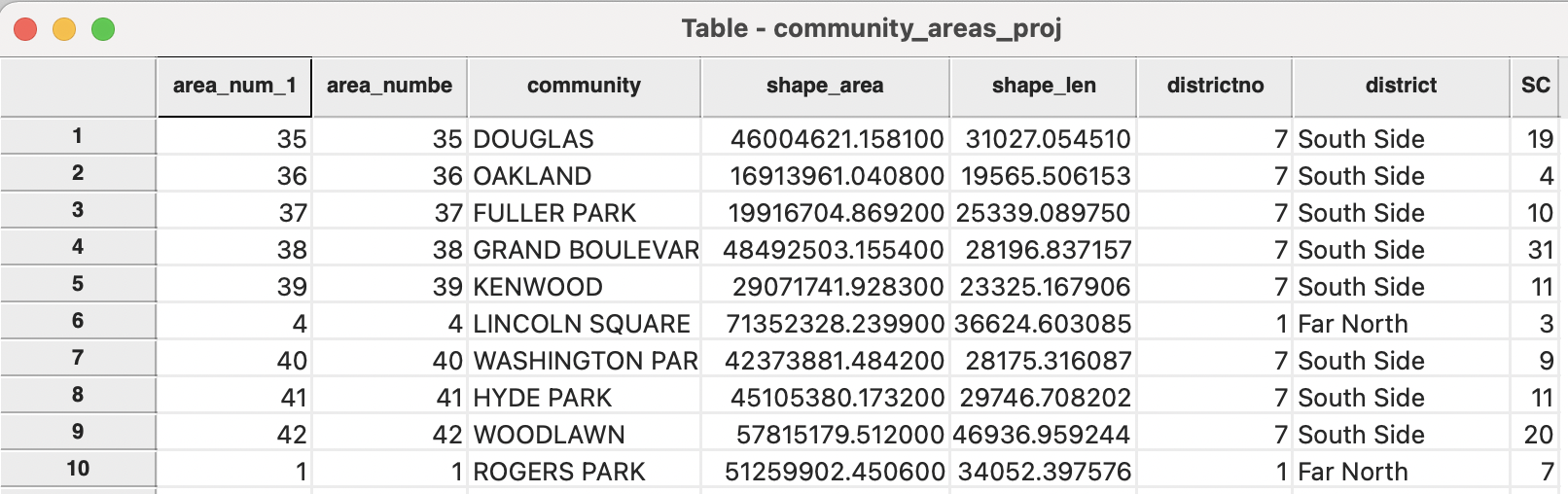
Figure 3.28: Spatial count in polygon area table
Alternatively, the opacity of the polygon layer can be reduced to zero to make the points visible.↩︎