4.6 Custom Classifications
So far, the classifications considered for the map legend have been endogenous, i.e., they were derived from the distribution of the variable under consideration (e.g., quantile, equal interval, natural breaks). However, such endogenous classification may not be that insightful when comparing the spatial pattern of different variables (on comparable scales, e.g., indices between 0 and 100), or when assessing the change in spatial pattern for a single variable over time. In addition, sometimes substantive concerns dictate the cut points, rather than data driven criteria. For example, this may be appropriate when specific income categories are attached to a policy. In those instances, the policy-based values for the classification are important, rather than what the internal data distribution would suggest.
When assessing the spatial distribution of a variable over time, the endogenous classifications are relative and re-computed for each time period, based on the variable distribution at that time. This can yield misleading impressions when the interest is in the evolution of the actual values. For example, when mapping crime rates over time, in an era of declining rates, the observations in the upper quartile in a later period may have crime rates that correspond to a much lower category in an earlier period. This would not be apparent using the endogenous classifications, but could be visualized by setting the same break points for each time period, i.e., an exogenous classification.
In GeoDa, this is accomplished through the Category Editor.
4.6.1 Category editor
The Category Editor is a complex tool that allows for the creation of a fully customized classification scheme. It can be invoked in a number of different ways. One option is to use the main menu, as Map > Custom Breaks > Create New Custom. A second way is as the bottom item from map options menu in Figure 4.2. Alternatively, the category editor can also be invoked directly by selecting the right-most icon on the toolbar in Figure 4.1.
4.6.1.1 Design
The custom categories are designed through the interface in Figure 4.17, shown after all editing has been completed. The initial settings and editing operations will be discussed below.
There are slight differences in the behavior of the dialog, depending on whether it is invoked from the toolbar, or as an option from an existing map. In the latter case, the associated map will be updated as a new classification is being developed. When invoked from the toolbar, there is nothing to update, but the initial variable may not be meaningful. It is the first variable in the data table, which is often just an identifier for each observations.
When the dialog opens (or at any point when the New button is selected), the first query is for the New Categories Title, where a name for the new classification must be specified (the default is Custom Breaks). In the example in Figure 4.17, Custom1 is the name of the new classification.
There are three major functions in the interface. First is the general definition of the classification, carried out through the items in the Create Custom Breaks panel at the top. This includes the naming of the categories, here Custom1.
The computations for the classification and their visualization in a histogram are based on the values for a specific variable, the Assoc Var., here sanitation. When the custom breaks are invoked from an existing map, the variable is entered automatically, but it is possible to change it from the drop down list.
As the breaks are edited, the impact on the associated histogram for the classification variable is shown instantly on the right hand side of the dialog.
Other important categories in the interface are whether the Breaks are User Defined (the default), or follow a traditional classification (Quantile, the default, Unique Values, Natural Breaks, or Equal Intervals). These choices may seem counter intuitive for a custom break editing operation, but it allows for the creation of custom labels for the categories (Section 4.6.1.3).
The Color Scheme for the legend is either sequential, diverging (the default), thematic (i.e., categorical) or custom. This provides an automatic selection of legend colors based on the ColorBrewer palettes. However, the color for each category can also be specified by clicking on its box below Edit Custom Breaks by means of the standard color editor (see Section 4.5.1). Finally, the number of Categories must be specified (the default is 4).33
In the example, in Figure 4.17, the color scheme has been set to sequential and the number of Categories to 5. The main effort consists of determining appropriate break points, which is considered next.
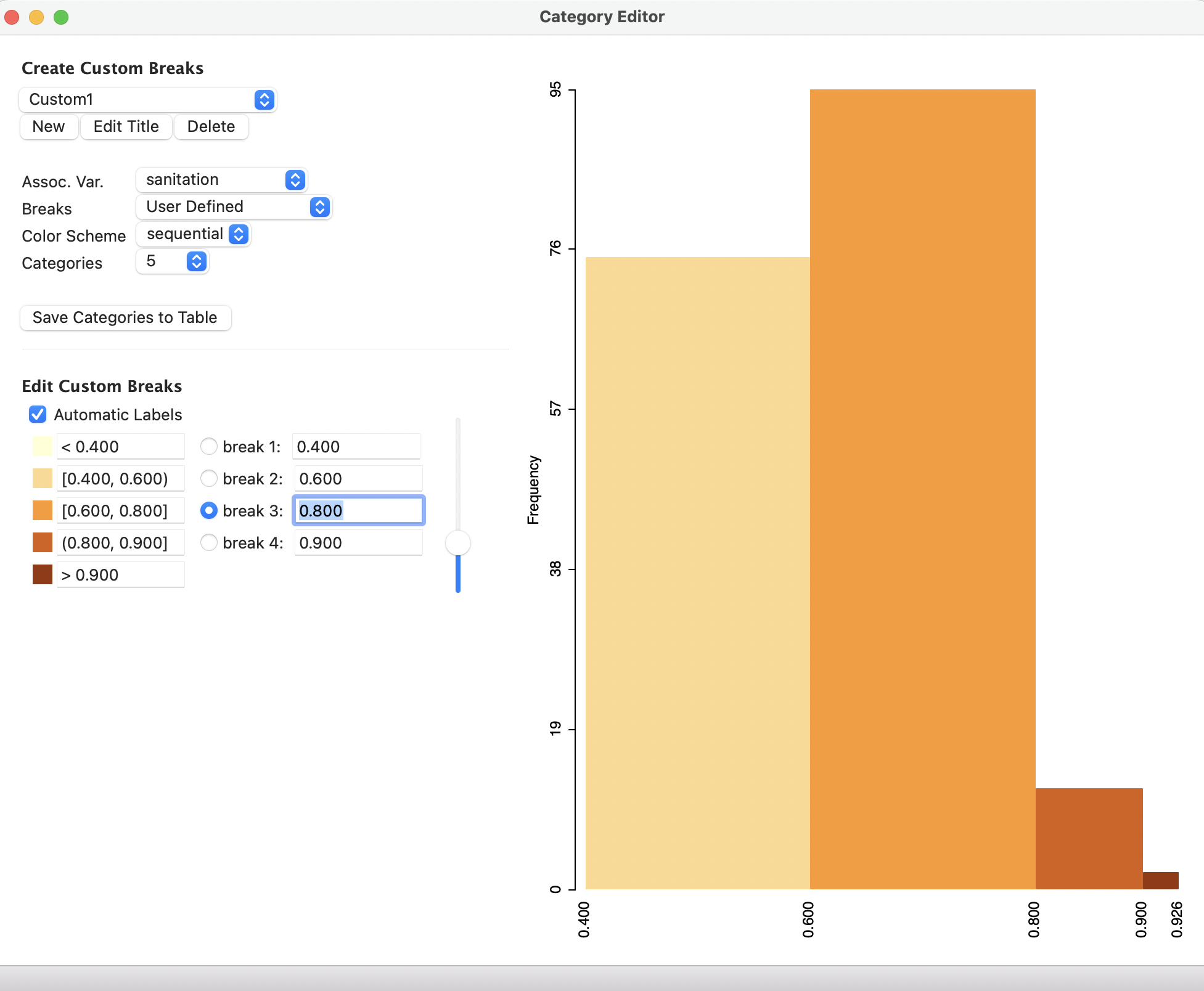
Figure 4.17: Category editor interface
4.6.1.2 Editing break points
The variable sanitation is a constructed index with values between 0 and 1. The observed range for the municipios in the State of Ceará goes from 0.417 to 0.926. These values are shown at, respectively, the left-most point and right-most point at the bottom of the histogram in Figure 4.17. An initial set of break points is suggested, which is almost never the final result. Instead of the suggested values, some absolute cut-offs must be entered, such as 0.4, 0.6, 0.8 and 0.9. This will allow for the comparison of the absolute position of each municipio across different variables, not just their relative position (which is produced by all endogenous classifications).
As new values for the break points are entered, the histogram is immediately updated. The values can be typed in, or obtained by moving the slider bar to the right.
The new break points are immediately associated with the specific custom break definition, without a saving operation. However, they can only be preserved through the use of a project file (see Section 4.6.3). The corresponding distribution is shown in the histogram in Figure 4.17.
4.6.2 Applications of custom categories
To illustrate the application of custom categories, consider the variables sanitation and infra (infrastructure). Both are obtained from the Brazilian Index of Urban Structure (IBEU) for 2013. They take on values from 0 to 1. The relative position of the municipios in Ceará on those two variables can be visualized by means of a quintile map, as in Figure 4.18. The spatial patterns are different, but some high performing municipios overlap.
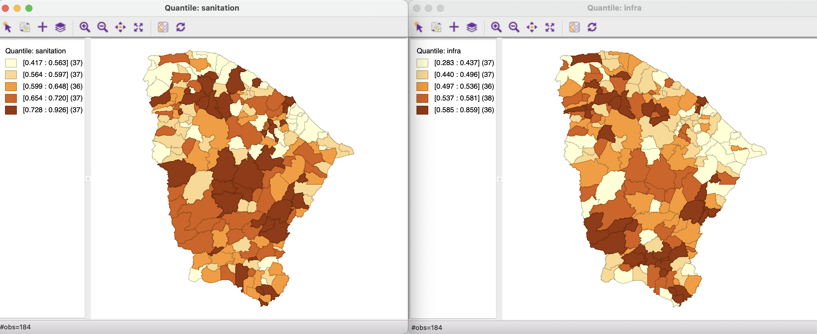
Figure 4.18: Quintile maps for sanitation and infrastructure
Contrast this pattern with the maps in Figure 4.19, based on the absolute cut-off points of 0.4, 0.6. 0.8 and 0.9. Clearly, the municipios do not perform as well on the infrastructure index as they do on the sanitation index. For example, the latter has 0 observations in the lowest category (< 0.4), whereas for infrastructure there are 16 such observations. Also, infrastructure has 0 municipios in the top category (> 0.9), whereas sanitation has 2. This allows for the comparison of not only the relative performance of the municipios, but also how they meet some absolute standards (admittedly arbitrary in this example).
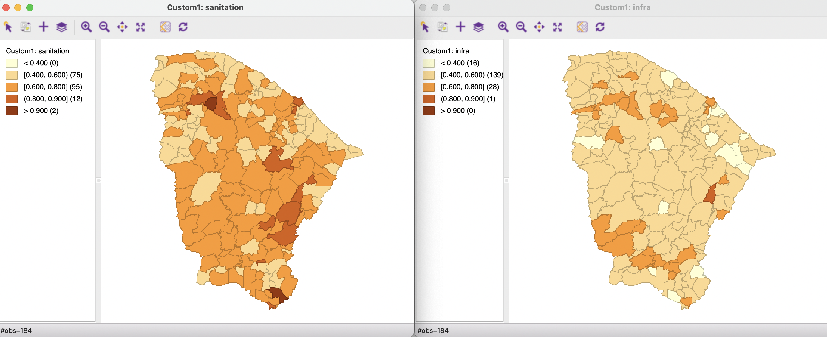
Figure 4.19: Thematic maps for sanitation and infrastructure using custom classification
4.6.3 Saving the custom categories - the Project File
When a project is closed, the information on the custom classification is lost, unless it is first saved in a so-called Project File. This file, associated with a geographic input layer, contains information on various variable transformations and other operations, most importantly dealing with spatial weights (see Chapter 10). It also contains the definition of any custom categories that were created. If this definition is not saved in a project file, then it will be lost, and will need to be recreated from scratch the next time the data set is analyzed.
The project file is created from the menu as File > Save Project. The file is saved with a file extension of gda. It is a text file that includes XML encoding. For example, a project file associated with the Ceará data could be zika_ceara.gda. Closer inspection reveals the section pertaining to custom_classifications in Figure 4.20.
The custom classification section contains all the aspects needed for the definition of the custom category.
When an analysis is started with the project file as input (e.g., instead of a shape file) then all transformations and custom categories become immediately available as an option for any map or histogram.
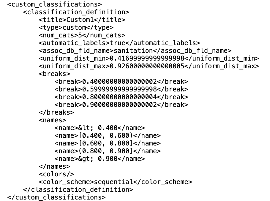
Figure 4.20: Custom category definition in project file
The classification can also be saved as a new variable in the table, using the Save Categories to Table button.↩︎