16.3 Local Moran
The Local Moran (Anselin 1995) is by far the most commonly used LISA statistic. It follows from a straightforward application to the global Moran statistic of the principles just outlined.
16.3.1 Formulation
As discussed in Chapter 13, the Moran’s I statistic is obtained as: \[\begin{equation} I = \frac{\sum_i \sum_j z_i.z_j.w_{ij} / S_0}{\sum_i z_i^2 / n}, \end{equation}\] with the variable of interest (\(z\)) expressed as deviations from the mean, and \(S_0\) as the sum of all the weights. In the row-standardized case, the latter equals the number of observations, \(n\). As a result, as shown in the discussion of the Moran scatter plot, the Moran’s I statistic simplifies to: \[I = \frac{\sum_i \sum_j w_{ij} z_iz_j}{\sum_i z_i^2}.\]
Using the logic just outlined, a corresponding Local Moran statistic would consist of the component in the double sum that corresponds to each observation \(i\), or: \[I_i = \frac{\sum_j w_{ij} z_iz_j}{\sum_i z_i^2}.\]
In this expression, the denominator is fixed and can thus further be ignored. To keep the notation simple, it can be replaced by \(a\), so that the Local Moran expression becomes \(a.\sum_j w_{ij} z_iz_j\). After some re-arranging, a simple expression is: \[I_i = a \times z_i \sum_j w_{ij} z_j,\] or, the (scaled) product of the value at location \(i\) with its spatial lag, the weighted sum or the average of the values at neighboring locations.
A special case occurs when the variable \(z\) is fully standardized. Then its variance \(\sum_i z_i^2/n = 1\), so that \(\sum_i z_i^2 = n\). Consequently, the global Moran’s I can be written as: \[I = \sum_i (a. z_i \sum_j w_{ij} z_j) = (1/n) \sum_i (z_i \sum_j w_{ij} z_j),\] or the average of the local Moran’s I. This case illustrates a direct connection between the local and the global Moran’s I.
Significance can be based on an analytical approximation, but, as argued in Anselin (1995), this is not very reliable in practice.113 A preferred approach consists of a conditional permutation method. This is similar to the permutation approach considered in the Moran scatter plot, except that the value of each \(z_i\) is held fixed at its location \(i\). The remaining n-1 z-values are then randomly permuted to yield a reference distribution for the local statistic, one for each location.
The randomization operates in the same fashion as for the global Moran’s I (see Section 13.5.2.2), except that the permutation is carried out for each observation in turn. The result is a pseudo p-value for each location, which can then be used to assess significance. Note that this notion of significance is not the standard one, and should not be interpreted that way (see the discussion in section 16.5).
Assessing significance in and of itself is not that useful for the Local Moran. However, when an indication of significance is combined with the quadrant location of each observation in the Moran Scatter plot, a very powerful interpretation becomes possible. The combined information allows for a classification of the significant locations as High-High and Low-Low spatial clusters, and High-Low and Low-High spatial outliers. It is important to keep in mind that the reference to high and low is relative to the mean of the variable, and should not be interpreted in an absolute sense. The notions of clusters and outliers are considered more in-depth in section 16.4.
16.3.2 Implementation
The Univariate Local Moran’s I is started from the Cluster Maps toolbar icon, the right-most icon in the spatial correlation group, highlighted in Figure 16.1. This brings up a drop down list, with the univariate Local Moran as the top-most item. Alternatively, this option can be selected from the main menu, as Space > Univariate Local Moran’s I.
Either approach brings up the familiar Variable Settings dialog which lists the available variables as well as the default weights file, at the bottom (e.g., oaxaca_q in the example). As in Chapter 14, the variable is p_PHA(2010), the 2010 percentage of the municipal population with access to health care. In the example, this variable is time enabled, which results in the selected year (2010) being listed in the dialog as well.
As a reference, a box map reflecting the spatial distribution of this variable is shown in the left-hand panel of Figure 14.1 (see also the left-hand panels in Figures 16.6 and 16.8 in this Chapter).
16.3.2.1 Significance map and cluster map
Clicking OK at this point brings up a dialog to select the number and types of graphs and maps to be created. The default is to provide just the Cluster Map, which is typically the most informative graphic. In addition, a Significance Map and a Moran Scatter Plot option is included as well.
To illustrate the Local Moran, selecting both cluster map and significance map brings up Figure 16.2. This visualizes the result of the default randomization test, using 999 permutations and a p-value cut-off of 0.05.
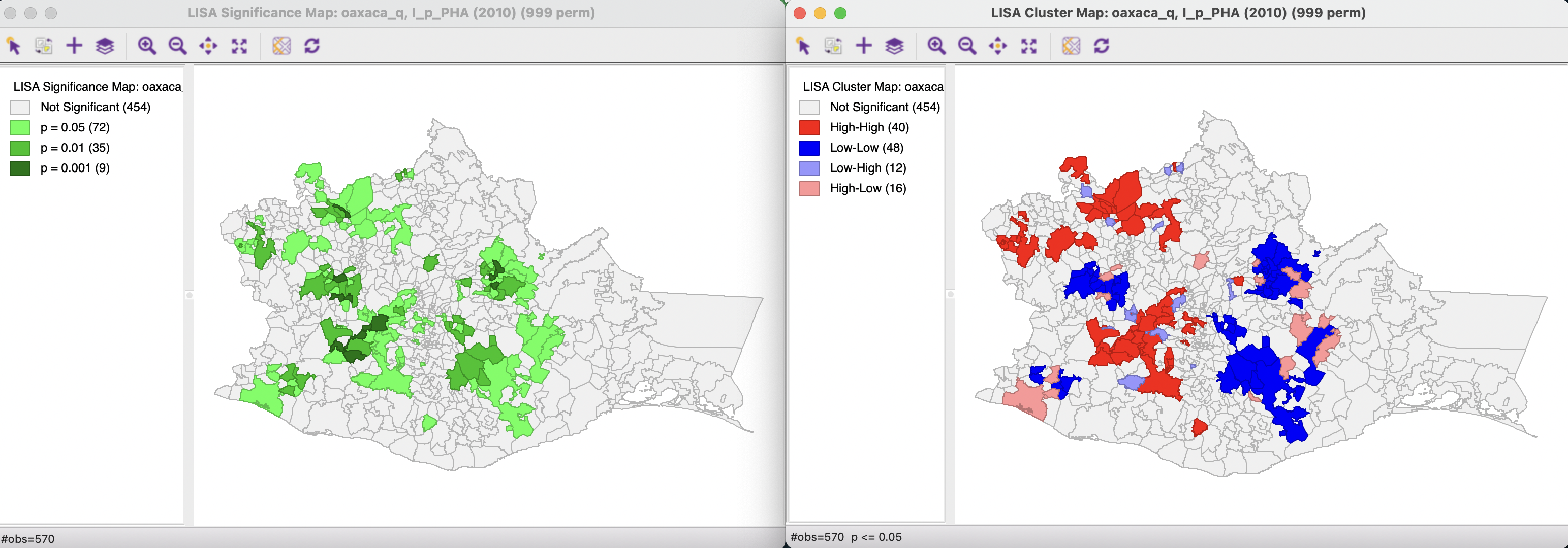
Figure 16.2: Significance Map and Cluster Map
The significance map on the left shows the locations with a significant local statistic, with the degree of significance reflected in increasingly darker shades of green. The map starts with p < 0.05 and shows all the categories of significance that are meaningful for the given number of permutations. In the example, since there were 999 permutations, the smallest pseudo p-value is 0.001, with nine such locations (the darkest shade of green).
The cluster map augments the significant locations with an indication of the type of spatial association, based on the location of the value and its spatial lag in the Moran scatter plot (see section 16.4). In this example, all four categories are represented, with dark red for the High-High clusters (40 in the example), dark blue for the Low-Low clusters (48 locations), light blue for the Low-High spatial outliers (12 locations), and light red for the High-Low spatial outliers (16 locations).
16.3.2.2 Randomization options
The Randomization option is the first item in the options menu for both the significance map and the cluster map. It operates in the same fashion as in the Moran scatter plot. As before, up to 99,999 permutations are possible (for each observation in turn), preferably using a specified random seed to allow replication.
The effect of the number of permutations is typically marginal relative to the default of 999. In the example, selecting 99,999 results in one more significant location (117 vs 116). As shown in the left-hand panel of Figure 16.3, there are now 70 locations significant at p < 0.05 (compared to 72), 34 locations at p < 0.01 (compared to 35), 11 locations at p < 0.001 (compared to 9), and one each at p < 0.0001 and p < 0.00001 (the smallest possible p-value). They are illustrated by different shades of green in the significance map.
The cluster map, in the right-hand panel, is similarly only marginally affected. There are two new observations in the High-High category, and one of the High-Low outliers disappears. Otherwise, the map is the same as for 999 permutations.
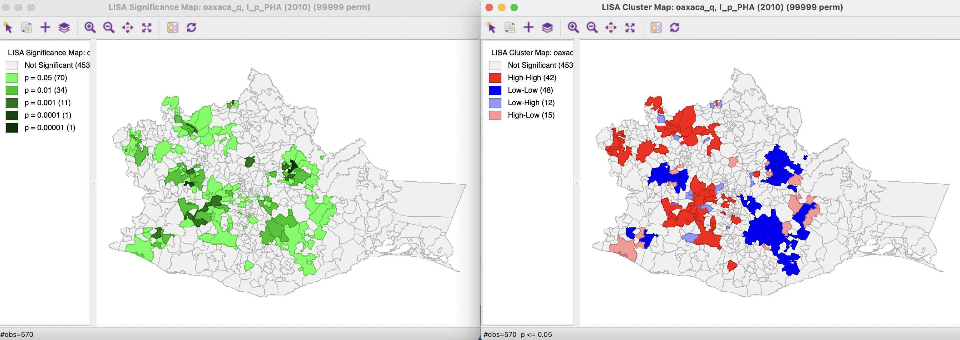
Figure 16.3: Significance Map and Cluster Map - 99999 permutations
16.3.2.3 Saving the Local Moran statistic
The third item in the options menu for the Local Moran is to Save Results.
This brings up a dialog with three potential variables to save to the table: Lisa Indices, Clusters and Significance. The default variable names are LISA_I, LISA_CL, and LISA_P. The first are the actual values for the local statistics, which are typically not that useful. The clusters are identified by an integer that designates the type of spatial association: 0 for non-significant (for the current selection of the cut-off p-value, e.g., 0.05 in the example), 1 for High-High, 2 for Low-Low, 3 for Low-High, and 4 for High-Low.
The default variable names would typically be changed, especially when more than one variable is considered in an analysis (or different spatial weights for the same variable).
16.3.2.4 Other options
In addition to the three options considered so far, there are several specialized operations for the cluster and significance map. These are covered in section 16.4 on clusters and spatial outliers (Select All) and 16.6 on conditional cluster maps (Show As Conditional Map).
The other options are customary, and include Selection Shape, Color and Show Status Bar, Save Selection, Copy Image to Clipboard, and Save Image As. In addition, when the data set is time-enabled, the Time Variable Options are available. Finally, the various options associated with the Connectivity item were covered in Section 10.4.5.1.
These other options operate in the same way as discussed before.