19.4 Co-Location Local Join Count Statistic

The second extension of the Local Join Count statistic to multiple variables considers co-location. This allows two or more variables to take a value of 1 at the same location, i.e., \(x_i = z_i = 1\).

For two variables, a co-location cluster requires that an observation for which \(x_i = z_i = 1\) coincides with neighbors for which \(x_j = z_j = 1\) as well. For two variables, the corresponding Local Join Count statistic takes the form (Anselin and Li 2019): \[CLC_i = x_iz_i \sum_j w_{ij}x_jz_j,\] with \(w_{ij}\) as unstandardized (binary) spatial weights. As before, there are \(P\) observations with \(x_i = 1\) and \(Q\) observations with \(z_i = 1\) out of a total of \(n\).

A conditional permutation approach can be constructed for those locations with \(x_i = z_i = 1\). The permutation consists of draws of \(k_i\) pairs of observations \((x_j, z_j)\) from the remaining set of \(n-1\) tuples, which contain \(P-1\) observations with \(x_j = 1\) and \(Q-1\) observations with \(z_j = 1\). In a one-sided test, the number of times are counted where the statistic equals or exceeds the observed join count value at \(i\).

The extension to more than two variables is mathematically straightforward. At each location \(i\), \(k\) variables are considered, i.e., \(x_{hi}\), for \(h = 1, \dots, k\), with \(\Pi_{h=1}^k x_{hi} = 1\), which enforces the co-location requirement.

The corresponding statistic is then: \[CLC_i = \Pi_{h=1}^k x_{hi} \sum_j w_{ij} \Pi_{h=1}^k x_{hj}.\] The implementation of a conditional permutation strategy follows as a direct generalization of the two-variable co-location case. However, for a large number of variables, such co-locations become less and less likely, and a different conceptual framework may be more appropriate.

19.4.1 Implementation

The Co-Location Local Join Count statistic is invoked from the third group in the drop down list associated with the Cluster Maps toolbar icon, or, from the menu, as Space > Co-location Local Join Count. This is followed by a Multi-Variable Settings dialog, where the variables to be considered can be specified. At the bottom of the dialog is the customary drop-down list with the spatial weights.

To illustrate this statistic, the two variables are Blk, tracts with majority Black population, and CAR, tracts where more than 50% of the commutes happen by car. The spatial weights are again queen contiguity, Chi_SDOH_q.

A co-location map of the two binary variables is shown in the left-hand panel of Figure 19.5. Of the 791 tracts, 167 are both majority Black and majority commute by car. Of the remainder, 254 are neither and 370 show a mismatch of the majorities. The corresponding Co-Location Local Join Count significance map is shown in the right-hand panel, using 99,999 permutations and a cut-off of 0.05. At 0.05, there are 90 cores of clusters that overlap, out of the 167, but at 0.01, only 57 of those remain. They confirm the impression of high dependence on commuting by car in majority Black neighborhoods.

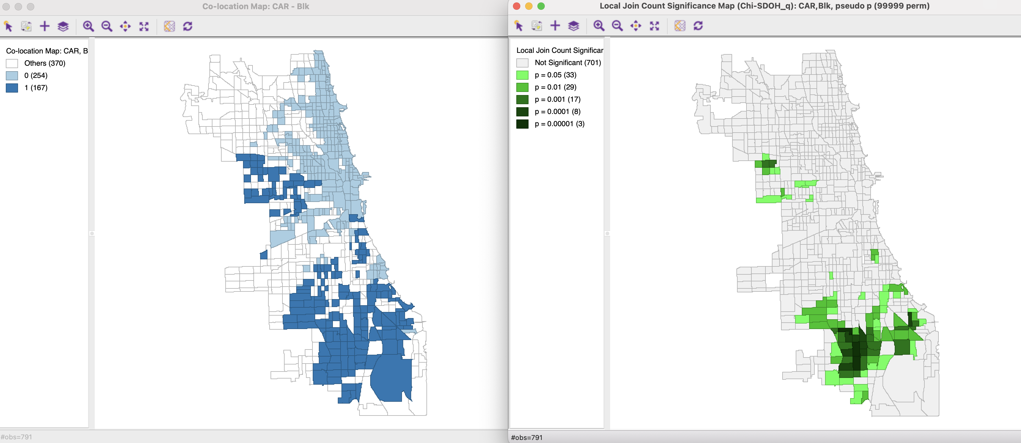
Figure 19.5: Co-Location Local Join Count

All the usual options are available.