15.3 Spatial correlogram
A spatial correlogram expresses the covariances or correlations between all pairs of observations as a function of the distance that separates them. The estimate is obtained from a non-parametric local regression fit, such as LOWESS (Section 7.3.2) or kernel regression. Its properties are based on the theory of nonparametric estimators of the autocovariance for a stationary random field, first outlined in Hall and Patil (1994; see also Bjornstad and Falck 2001).
With the variables expressed in standardized form as \(z\), this approach boils down to a local regression: \[z_i.z_j = g(d_{ij}) + \epsilon,\] where \(d_{ij}\) is the distance between a pair of locations \(i, j\), \(\epsilon\) is an error term, and \(g\) is the non-parametric function to be determined from the data. Since the variables are standardized, the result is a spatial correlogram which shows how the strength of correlation varies with the distance separating the observations.
In GeoDa, this is implemented by first arranging pairs of observations by distance bin, similar to the approach taken in the estimation of a semi-variogram in geostatistics. The correlogram is then the nonlinear curve fit to the
average correlation for all pairs of observations
in a distance bin by means of a LOWESS regression .
The main interest in the spatial correlogram is to determine the range of interaction, i.e., the distance within which the spatial correlation is positive. In addition, following Tobler’s law (Tobler 1970), the strength of the correlation should decrease with distance.
Beyond the range of interaction, the correlation should become negligible, although in practice it can still show fluctuations.107
15.3.1 Creating a spatial correlogram
To illustrate the spatial correlogram, I use the Italy Community Banks sample data set from Chapter 11 in time-enabled form. Specifically, the spatial pattern of the loan loss provisions over customer loans is investigated for 2016 (LLP (2016)). The presumption is that this variable addresses similar local risk environments, which would suggest spatial autocorrelation.
A quantile map with eight categories is shown in Figure 15.2. The suggestion of patterning is confirmed by a Moran’s I of 0.179, with associated z-value of 5.41 (based on 999 permutations) for the six neighbor k-nearest neighbor weights truncated at 73 km (italy_banks_te_d73_k6.gal).108
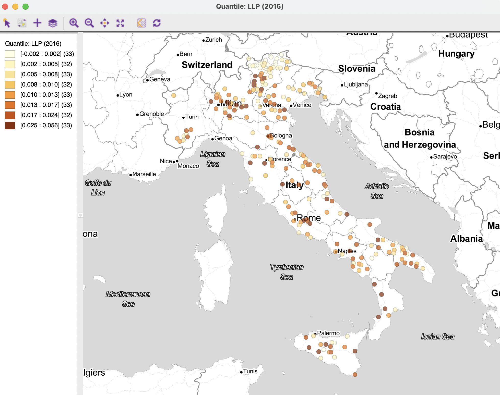
Figure 15.2: Spatial distribution of loan loss provisions - Italian banks 2016
The spatial correlogram functionality is invoked by selecting the middle icon in the spatial analysis group, as in Figure 15.1, and choosing Spatial Correlogram. Alternatively, from the menu, it can be started by selecting Space > Spatial Correlogram (the item near the very bottom of the list of options).
This brings up a Correlogram Parameters dialog with the default parameter settings and a graph in the background. However, this initial graph is almost never informative at this point, since it shows a correlogram for the first variable, which is usually an ID value.
The initial layout of the interface is shown in the left-hand panel of Figure 15.3. The items at the top of the dialog are the Variable (available from a drop down list), the Distance metric (default is Euclidean Distance, but Arc Distance is also available, expressed either as miles or as kilometers). In the example, since the data set is time enabled, the Variable also has an associated Time drop down list. For the initial default setting, LLP (2016) and 2016 are used with Euclidean Distance (given the projection used, this distance is in meters).
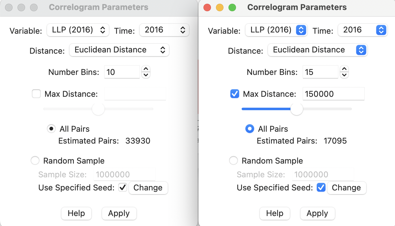
Figure 15.3: Correlogram parameter selection
Next follows the Number of Bins. The non-parametric correlogram is computed by means of a local regression on the spatial correlation estimated from the pairs that fall within each distance bin. The number of bins determines the distance range of each bin. This range is the maximum distance divided by the number of bins. The more bins are chosen, the more fine-grained the correlogram will be. However, this also potentially can lead to too few pairs in some bins (the rule of thumb is to have at least 30).
The number of pairs contained in each bin is a result of the interplay between the number of bins and the maximum distance. As the default, All Pairs are used, with Max Distance unchecked. In the example, with 261 observations, this yields: \([261^2 - 261]/2\) = 33930 pairs, as listed in the Estimated Pairs box.
In many instances in practice, using all pairs may not be a good choice. For example, when there are many observations, the number of pairs quickly becomes unwieldy and the program will run out of memory. Also, the correlations computed for pairs that are far apart are not that meaningful, since they should be zero due to Tobler’s law. Therefore it is often practical to truncate the observations to only those pairs that are within a reasonable distance range.
The bottom half of the dialog provides options for fine-tuning these choices. These are considered in Sections 15.3.2.1 and 15.3.2.2.
With the default set as in the left-hand panel of Figure 15.3, the spatial correlogram shown in Figure 15.4 is created.
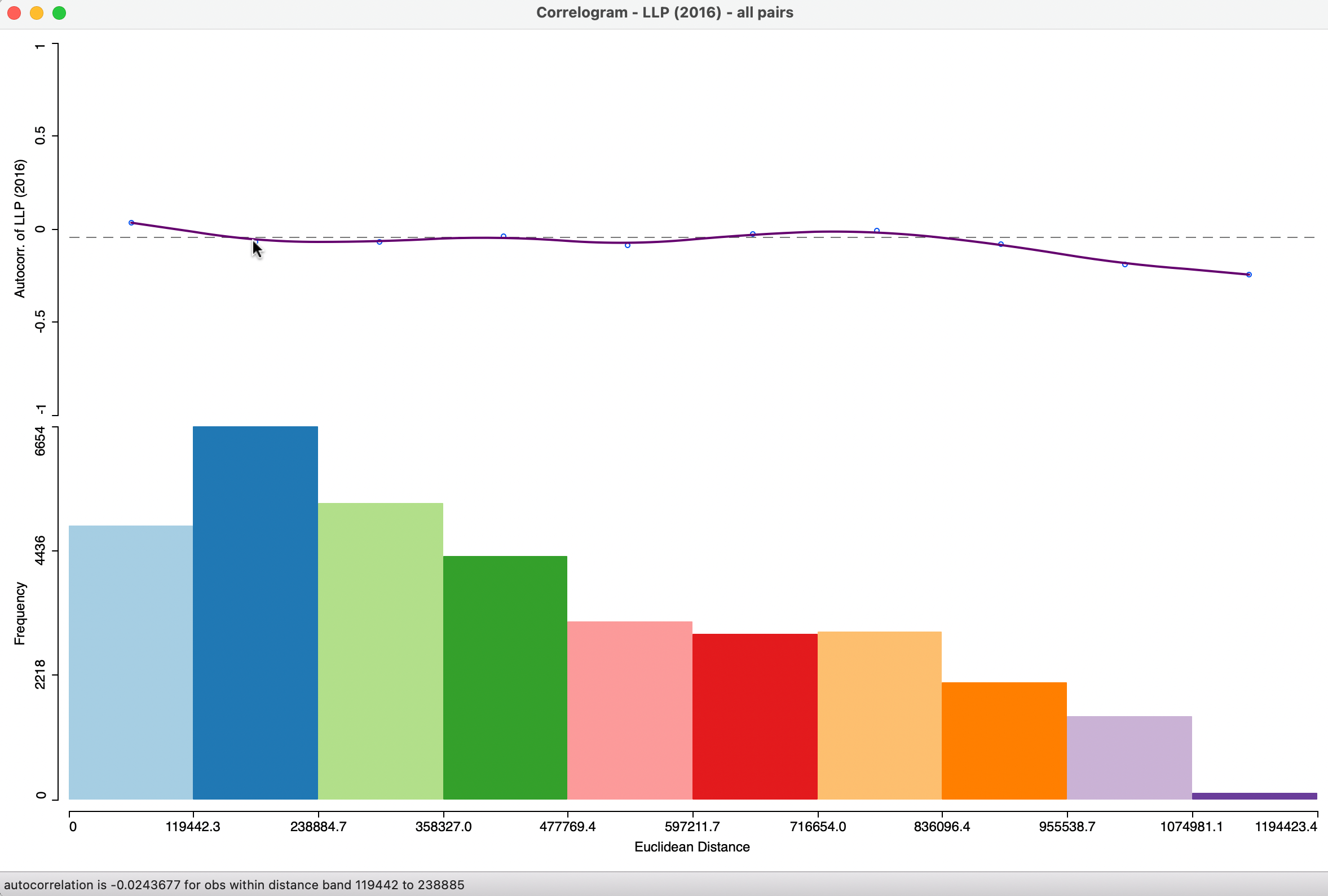
Figure 15.4: Default spatial correlogram - LLP (2016)
15.3.1.1 Interpretation
The top half of the graph in Figure 15.4 is the actual correlogram that depicts how the spatial autocorrelation changes with distance. Hovering the pointer over each blue dot gives the spatial autocorrelation associated with that distance band in the status bar. For example, the second dot corresponds with an autocorrelation of -0.024 for observations within the distance band from 119.4 km to 238.9 km, as shown in the status bar (the distances in the graph are expressed in meters). The first dot corresponds with an autocorrelation of 0.081.
The intersection between the correlogram and the dashed zero axis, which determines the range of spatial autocorrelation, happens in the midpoint of the second range, or roughly around 179 km. Beyond that range, the autocorrelation fluctuates around the zero line.
The bottom half of the graph consists of a histogram that shows the number of pairs of observations in each bin. Hovering the pointer over a given bin shows in the status bar how many pairs are contained in the bin. In the example, each bin has more than sufficient observation pairs. Even the last bin, which seems small (a function of the vertical scale), contains 102 pairs to compute the average autocorrelation.
15.3.2 Spatial correlogram options
The spatial correlogram has four main options, invoked in the usual way by right clicking on the graph.
The Change Parameters item brings back the Correlogram Parameters dialog and allows for fine tuning of the number of bins, maximum distance and randomization options (Sections 15.3.2.1 and 15.3.2.2).
The Edit LOWESS Parameters option manipulates the bandwidth and other technical parameters that can be specified for any LOWESS smoother. The default is to use a bandwidth of 0.20, which works well in most situations. As usual, a larger bandwidth will yield a (slightly) smoother curve, and a smaller bandwidth will work in the opposite way. This option works in exactly the same manner as for the standard LOWESS nonlinear smoother (Section 7.3.2.1).
The View > Display Statistics option generates a list of descriptive statistics for each bin. The computed autocorrelation is provided, as well as the distance range for the bin (lower and upper bound), and the number of pairs used to compute the statistic. In addition, there is a summary with the minimum and maximum distance, the total number of pairs, and an estimate for the range, i.e., the distance at which the estimated autocorrelation first becomes zero (see the discussion of Figures 15.5 and 15.6 for an illustration). The other View options are the familiar Set Display Precision, Set Display Precision on Axes and Show Status Bar. The latter is active by default.
Finally, Save Results provides a record of the descriptive statistics of the correlogram in a text file (with file extension csv). The file contains the information listed at the bottom of the graph when View > Display Statistics has been selected, with a column matching each bin. The file includes the estimates of the spatial autocorrelation, bin ranges, number of observations in each bin, as well as the summary.
15.3.2.1 Maximum distance and number of bins
In most situations in practice, the default use of all the distance pairs is not informative. In addition, there is a good reason to limit the maximum distance considered in the selection of pairs, since correlations at large(r) distances are both sparser (fewer pairs in a bin, which leads to less precise estimates) and supposed to be near zero (Tobler’s law).
The Correlogram Parameters dialog contains options to set the Max Distance. When this option is checked, half of the largest inter-observation distance is used.109 In the example, that would be about 597 km, resulting in 17095 Estimated Pairs, about half of the number when all pairs are used (not shown).110
Instead of using a rule of thumb such as half the total distance, the maximum distance can be specified explicitly, as in the right-hand panel of Figure 15.3. Here, a value of 150000 (150 km) is entered. Combined with the default Number Bins of 10, and with View > Display Statistics activated, this yields the correlogram in Figure 15.5.
The graph header lists the cutoff, but also gives that all pairs have been used. This should be interpreted in the sense that all pairs that meet the distance cutoff are used in the computations, as opposed to a random sample (Section 15.3.2.2).
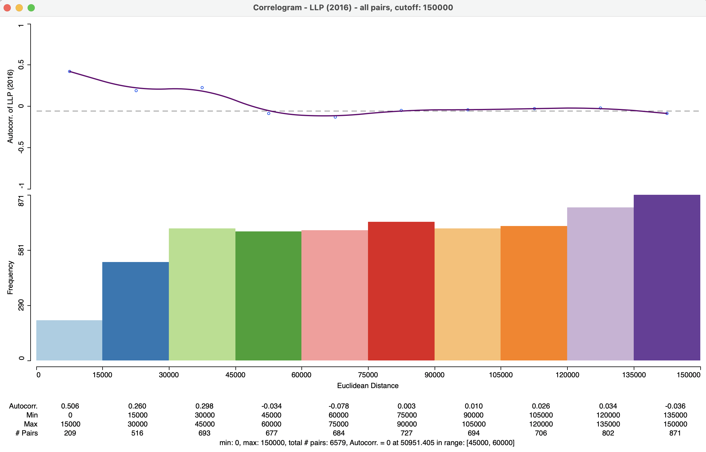
Figure 15.5: Spatial correlogram - LLP, 150km cut off, 10 bins
The distance range for each bin is now 15 km (15000 in the graph) and, as a result, the range is estimated to be between 45 km and 60 km, contrasted with more than double the figure obtained in Figure 15.4. Also, the initial spatial autocorrelation, for pairs within 15km of each other is 0.506, compared to 0.081 for the first range in the default setting. The descriptive statistics depict the change of the estimated autocorrelation coefficient with distance at a much more fine grained level than before. The correlogram shows the desired shape, decreasing with distance until the range is reached, and more or less flat afterwards. The computations are based on 6,579 pairs, less than a fifth of the original total.
A further refinement can be obtained by increasing the number of bins for the same maximum distance. In Figure 15.6, the correlogram is depicted for 15 bins with the 150 km cut-off (the settings shown in the right-hand panel of Figure 15.3), resulting in a range of 10 km for each bin. The zero autocorrelation is estimated to occur between 50 and 60 km, an even narrower band than for Figure 15.5. The autocorrelation in the first 10 km range is 0.503, basically the same as in the first 15 km range shown before. The overall shape of the correlogram also remains the same.
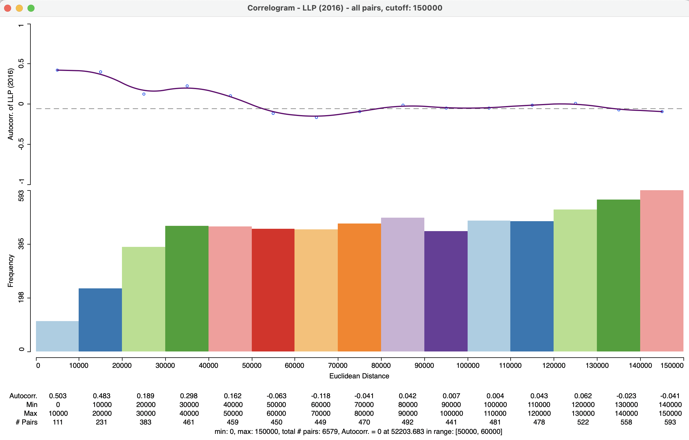
Figure 15.6: Spatial correlogram - LLP, 150km cut off, 15 bins
Overall, this suggests quite a strong pattern of positive spatial autocorrelation at short distances, but negligible association beyond distances of 60 km. This highlights a different aspect of spatial autocorrelation than can be provided by a statistic like Moran’s I, which considers all pairs that meet the spatial weights criterion.
15.3.2.2 Random sampling
A final feature of the correlogram is the ability to compute the spatial correlations for a sample of locations, which reduces the number of pairs used in the calculations. This is especially useful when the data set is large, in which case the number of pairs could quickly become prohibitive.
In the example used here, this is not really necessary, since the default sample size of 1,000,000 that is used to generate the random sample exceeds the current total number of pairs in the data set. To implement this option, the Random Sample radio button needs to be checked and a sample size specified if the default of 1 million is not desired. Also, to allow exact replication, the Use Specified Seed option should be checked (the seed can be adjusted by means of the Change button).
In practice, the sampling approximation is quite good, as long as the selected sample size is not too small relative to the original data size.
Some autoregressive spatial processes induce a pattern of alternating positive and negative autocorrelations, but a further consideration of this is beyond the current scope.↩︎
The Moran scatter plot calculation in
GeoDaremoves the two isolates from the computations.↩︎This follows one of the most common rules of thumb from geostatistics, e.g., as in Journel and Huijbregts (1978) and Deutsch and Journel (1998).↩︎
Since the estimated number of pairs is computed on the fly, as the maximum distance is adjusted by means of the slider, it is only an approximation. The actual number of pairs used in the calculation of the pairwise correlations is given in the status bar of the correlogram.↩︎