14.4 The many faces of space-time correlation
In contrast to the univariate Moran scatter plot, where the interpretation of the linear fit is unequivocally Moran’s I, there is no such clarity in the bivariate case. In addition to the interpretation offered above, which is a traditional Moran’s I-like coefficient, there are at least four additional perspectives that are relevant. Each is briefly considered in turn.
14.4.1 Serial (temporal) correlation
A first interpretation is the regression/correlation between the variable under consideration at two points in time, i.e., the linear relationship between \(z_{i,t}\) and its time lag \(z_{i,t-1}\). Since all variables are expressed as standardized entities, regression and correlation are equivalent.105
The result for the relationship between p_PHA (2020) and p_PHA (2010) is shown in Figure 14.7. The slope of the regression line is slightly positive and highly significant (p-value of 0.000) at 0.157. This suggests an overall positive correlation between the values at the two points in time. However, the overall fit of the regression is very poor, with an \(R^2\) of only 0.025.
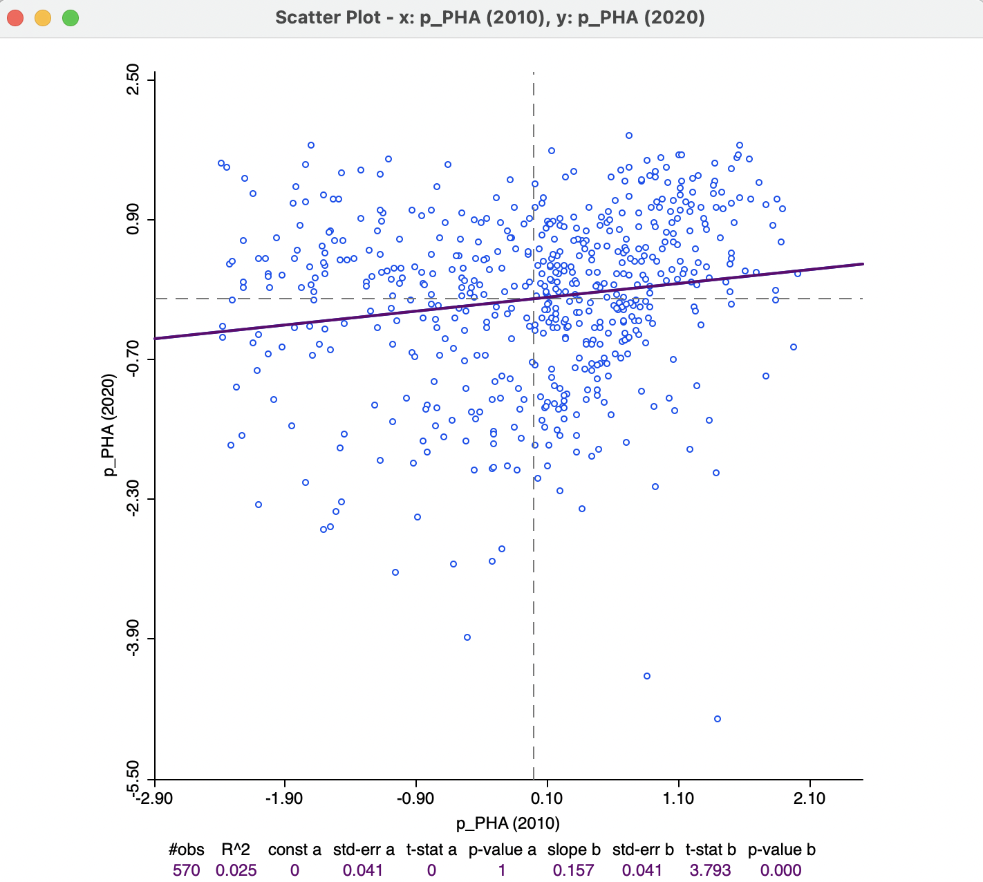
Figure 14.7: Correlation between access to health care in 2020 2010
14.4.2 Serial (temporal) correlation between spatial lags
A second perspective is the linear relation between the spatial lag of the variable of interest between the two time periods, i.e., a regression of the variable \(\sum_j w_{ij} y_{j,t}\) on \(\sum_j w_{ij} y_{j,t-1}\), or W_pPHA (2020) on W_pPHA (2010). In some sense, if there is a strong temporal correlation between the variable in-situ, as well as spatial correlation in each of the time periods, one may expect a temporal correlation between their neighbors in the form of the associated spatial lags. However, this assumes that the location of the clusters in unchanging over time, a property that the global Moran’s I is unable to assess.
The result is shown in Figure 14.8. The regression slope of 0.073 is not significant, with a p-value of 0.132. Also, the overall fit is very poor, given the \(R^2\) of 0.004. This is no surprise, given the ball-like shape of the scatter plot. In other words, while there is a relationship between the health access for two different time periods, this does not hold for the neighbors (spatial lags). This finding provides additional support for the notion that the clusters in the two years may be in different locations. If they were in the same locations, then the spatial lags for the two time periods would tend to be correlated.
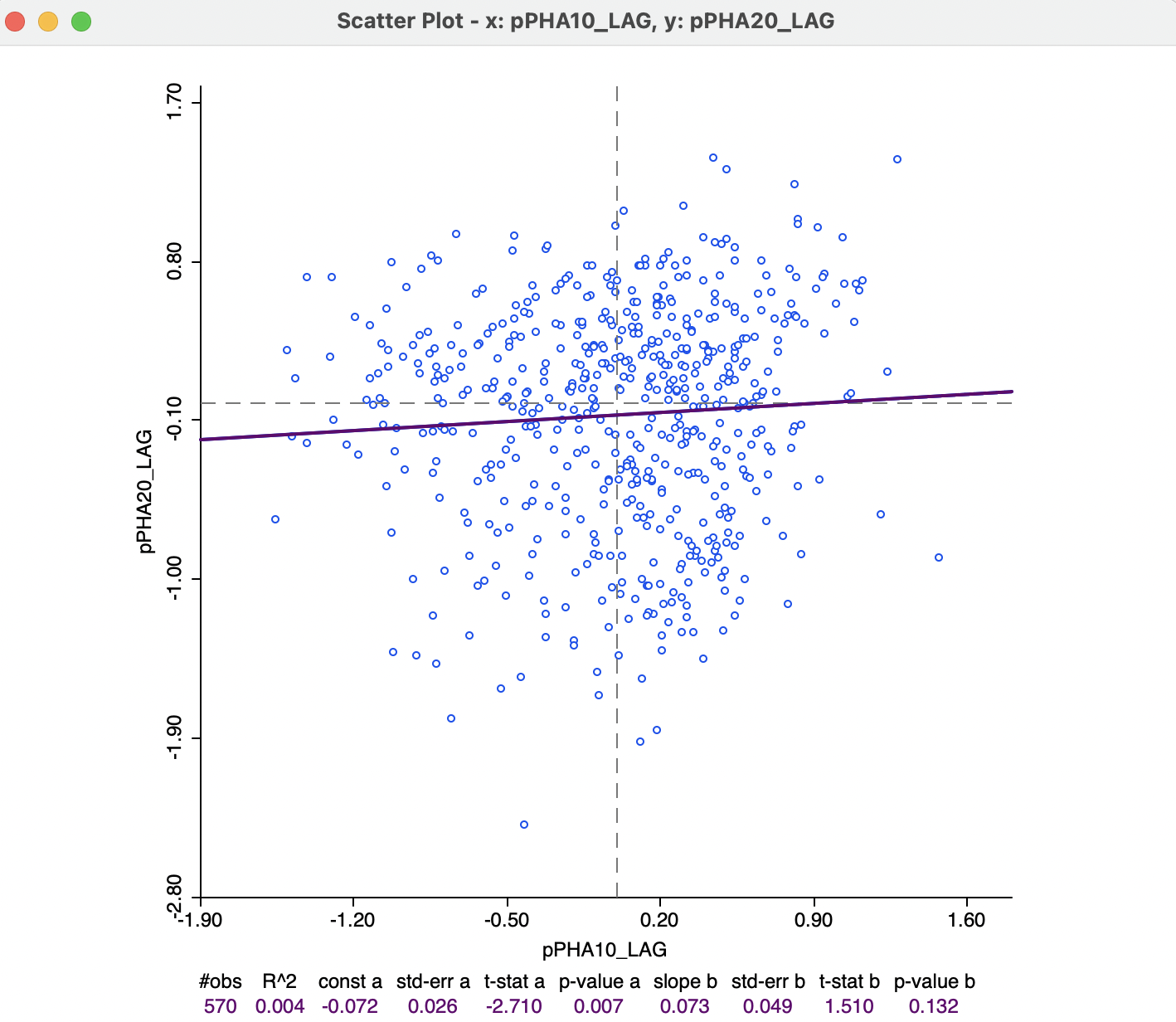
Figure 14.8: Correlation between the spatial lag of access to health care in 2020 and the spatial lag in 2010
14.4.3 Space-time regression
A third perspective is offered by a regression of the value of a variable at time \(t\) on the value of its neighbors at time \(t - 1\), formally, a regression of \(y_{i,t}\) on \(\sum_j w_{ij} y_{j,t-1}\). This is the most natural formulation of a space-time regression, expressing how the values at neighboring locations at the previous time period diffuse to the location at the next time period.
In Figure 14.9, this is illustrated for a regression of p_PHA (2020) on W_pPHA (2010). Again, the scatter plot is highly circular, yielding an almost horizontal slope for the linear fit. The regression coefficient of -0.028 is not significant, with a p-value of 0.718. The \(R^2\) is actually zero!
In other words, here we find no direct relationship between the value at a location and its neighbors in a previous location, consistent with the lack of significance of the bivariate Moran’s I in Figure 14.6.
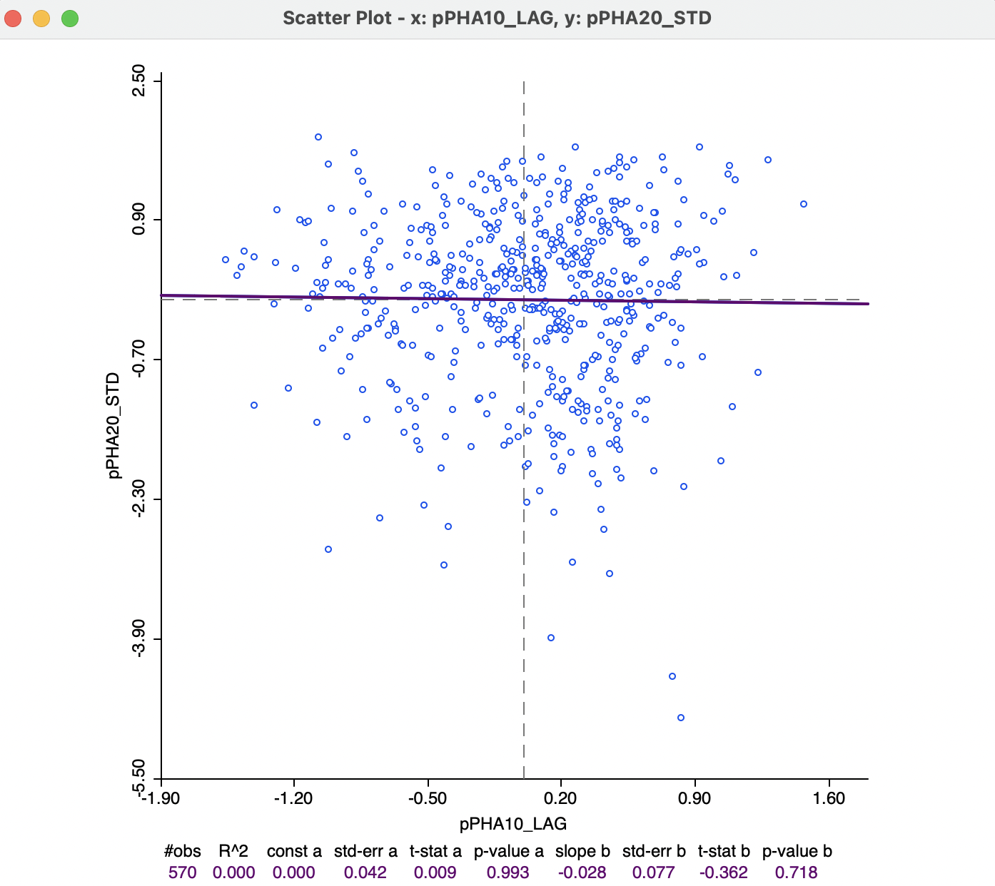
Figure 14.9: Correlation between access to health care in 2020 and its spatial lag in 2010
14.4.4 Serial and space-time regression
A final perspective is offered by including both in-situ correlation and space-time correlation in a regression specification. Specifically, this is expressed as a regression of \(y_{i,t}\) on both \(x_{i,t-1}\) and \(\sum_j w_{ij}x_{j,t-1}\). In the absence of temporal error autocorrelation, standard ordinary least squares regression will yield unbiased estimates of the coefficients.
The results for a regression of p_PHA (2020) on p_PHA (2010) and W_pPHA (2010) are shown in Figure 14.10. All variables are in standardized form. Purely as an illustration, this uses the regression functionality of GeoDa, a discussion of which is beyond the scope of this book.106
The specification offers yet a different perspective on the space-time relationships. Both regression coefficients are significant, but the coefficient of the space-time lag is negative and only weakly significant, with a p-value of 0.04. The overall adjusted \(R^2\) is only 0.03. This would suggest that after correcting for in-situ correlation, the effect of neighbors in the past was negative, rather than positive.
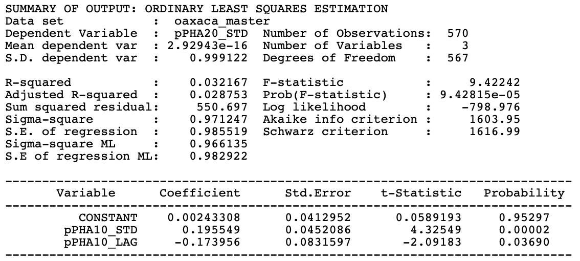
Figure 14.10: OLS regression of pPHA 2020 on pPHA 2010 and W PHA 2010
Needless to say, focusing the analysis solely on the bivariate Moran scatter plot provides only a limited perspective on the complexity of the dynamics of space-time patterns. In practice, the full space-time regression may provide the most reliable insights.
The regression can be carried out by selecting Data > View Standardized Data in the scatter plot, or by using the saved standardized values and their spatial lags from the Moran scatter plot for each individual year (by means of the Save Results option).↩︎
See Anselin and Rey (2014) for specifics on both the methods and their implementation in
GeoDa.↩︎