11.6 Manipulating Weights
The information in spatial weights can be manipulated in a limited number of ways. Set operations allow the creation of a new set of weights by union or intersection operations on two existing weights files. In addition, asymmetric weights, typically k-nearest neighbor weights, can be made symmetric.
11.6.1 Set operations
Once multiple weights are included in the Weights Manager, it becomes possible to carry out set operations on any pair. With two weights selected, say italy_banks_te_d73 (for a distance band of 73 km) and italy_banks_te_k6 (for 6 k-nearest neighbors), the buttons Intersection and Union become active (placed directly above Property in the dialog).
Figure 11.19 shows the graph structure that results when these two weights are combined through an Intersection operation.85 The only links that remain are those where some of the six nearest neighbors fall within 73 km. The new structure illustrates how some of the drawbacks of the individual weights were remedied.
The very dense connections in the north, shown in Figure 11.9, become much sparser, since only six of the distance-band neighbors are retained. On the other hand, the artificial connections in the k-nearest neighbor graph in Figure 11.11 are removed by imposing a 73 km distance constraint. This yields the same two isolates as for the original distance-band, highlighted in the figure.
Nevertheless, the resulting compromise provides a better reflection of potential interaction pairs for the community banks.
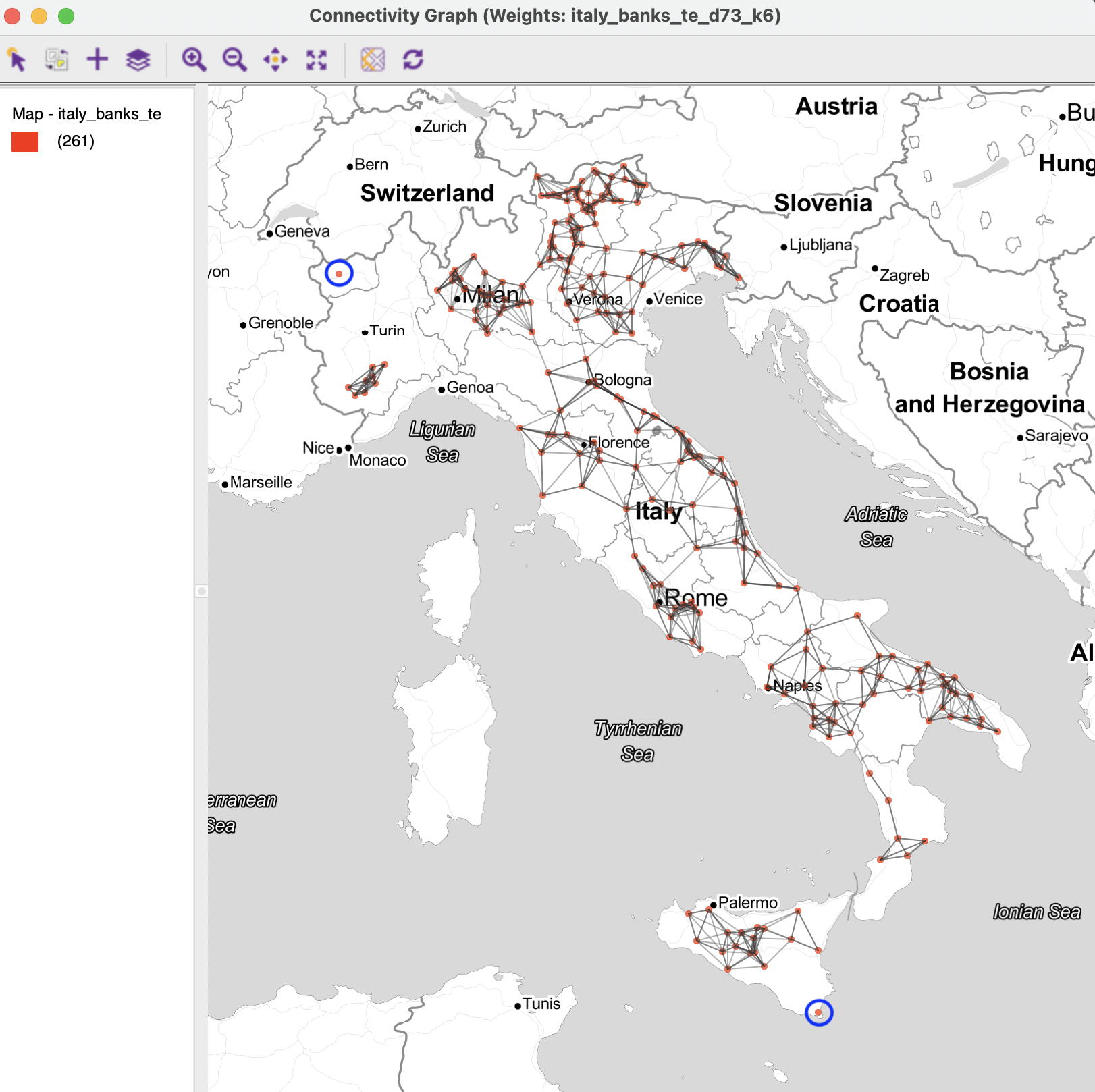
Figure 11.19: Connectivity graph for intersection distance 73km and knn 6
The Union function operates in a similar way (again, two weights need to be selected to activate this functionality). An obvious application would be to combine pure first and second order contiguity weights, although this functionality is built-in through the Include lower orders option for contiguity weights.
11.6.2 Make symmetric
As discussed in Section 11.3.2, there are two straightforward ways to turn an asymmetric k-nearest neighbor matrix into a symmetric one. One approach is inclusive and identifies a link as long as either \(w_{ij}\) or \(w_{ji}\) is non-zero. This is the default solution activated when the Make Symmetric button is selected in the Weights Manager. As a result, the new symmetric weights will be denser than the original k-nearest neighbor weights.
The second approach is exclusive in that a link is only counted when it exists in both directions: \(w_{ij} = w_{ji} = 1\). This is activated when the mutual box is checked, next to the Make Symmetric button. The resulting symmetric weights will be sparser than the original k-nearest neighbor weights.
For example, when applied to the 6 k-nearest neighbor weights for the Italian community banks, the inclusive symmetric weights have neighbors ranging from 6 to 13 (clearly, the minimum will be 6, as in the original weights, but the maximum can be more than 6). The median number of neighbors has increased to 7, with an overall density of 2.8 /%.
In contrast, the exclusive criterion yields weights with 0 to 6 neighbors (in this case, 6 is the maximum), and thus creates some isolates. The median number of neighbors has decreased to 5, with an overall density of 1.73 /%.
Which of these transformation is appropriate, will depend on each specific empirical circumstance. As a rule, a careful consideration of the weights characteristics is strongly recommended, especially by means of the connectivity graph.
Finally, it is important to save the created weights in a Project File, so that metadata can be preserved in later analyses.