3.5 Aggregation
Spatial data sets often contain identifiers of larger encompassing units, such as the state that a county belongs to, or the census tract that contains individual household data. Such nested spatial scales readily lend themselves to aggregation to the larger unit. The aggregation computes observations for the new spatial scale as the sum, average or other operation applied to the values at the lower scale. Note that this only makes sense if the underlying variables are spatially extensive, such as counts (total population, total households). Without proper re-weighting, the aggregation gives misleading results for variables expressed as medians or percentages (e.g., median household value, median income).
GeoDa supports two different ways to compute aggregates from the smaller units.
One approach also creates a dissolved layer, i.e., a spatial layer that includes both a map for the larger spatial units and a data table with the corresponding aggregated observations. The second approach
is limited to computing a new table with the aggregate information. It does not generate a spatial component.
3.5.1 Dissolve
The Dissolve functionality is part of the Tools menu (Tools > Dissolve), or can be accessed by selecting the Dissolve option from the Tools icon on the toolbar, the right-most icon in Figure 2.1.
To illustrate this feature, the point of departure is the merged data set created in Section 2.4.3 (e.g., saved as Chicago_2020.shp). This data set contains socio-economic data for the 77 Chicago community areas. In addition, it also has an identifier that associates each community area with a larger encompassing district, i.e., the variable districtno. The corresponding layout is given by the themeless base map from Figure 2.4
The dialog, shown in 3.16, requests three important pieces of information. The most critical is the variable for dissolving, i.e., the key that indicates the larger scale to which the observations will be aggregated (here, districtno). Next follows the selection of the variables for which the aggregate values will be calculated. In the example in Figure 3.16, these are 2000_POP, 2010_POP and TOT_POP (the population in 2020 from ACS). The variables are selected by double clicking on them, or by selecting them and then using the > key to move them to the right-hand side column.
Finally, we need the proper aggregation Method must be selected. The available options are Count, Average, Max, Min, and Sum. The Count function doesn’t actually compute any aggregate values, but provides a count of the number of smaller units included in the larger unit (e.g., the number of community areas in each district). For example, Sum will yield the population totals for each district.
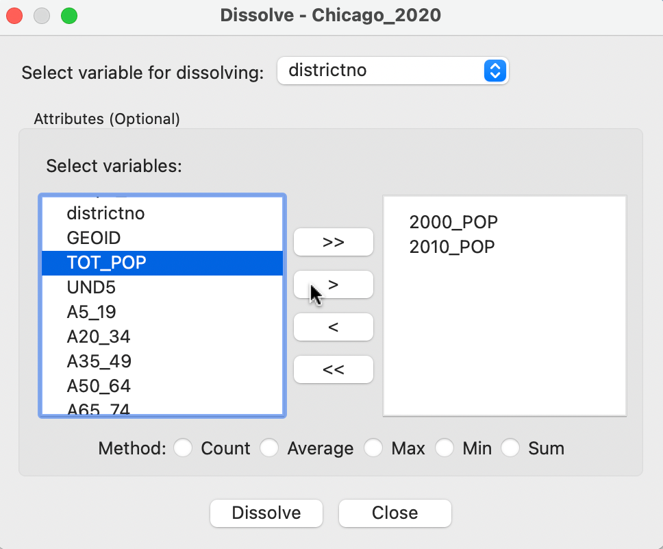
Figure 3.16: Dissolve dialog
After activating the Dissolve button, the usual file creation dialog is produced to specify a file type and file name, e.g., Chicago_district_2020.shp.
Figure 3.17 shows the outline of the nine districts (in red), together with the original community area boundaries (in blue). This is an illustration of a multiple layer operation, since both the community area layer and the district layer are combined on the same map. The multilayer functionality is further detailed in Section 3.6.1.
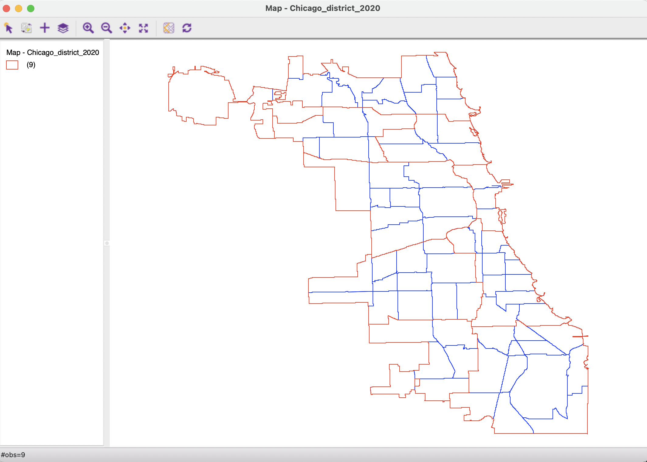
Figure 3.17: Dissolved districts map
The associated table (Figure 3.18) lists the population totals in the three census years for the district aggregates. The table also includes a new variable, AGG_COUNT, which indicates the number of community areas aggregated into the respective district.
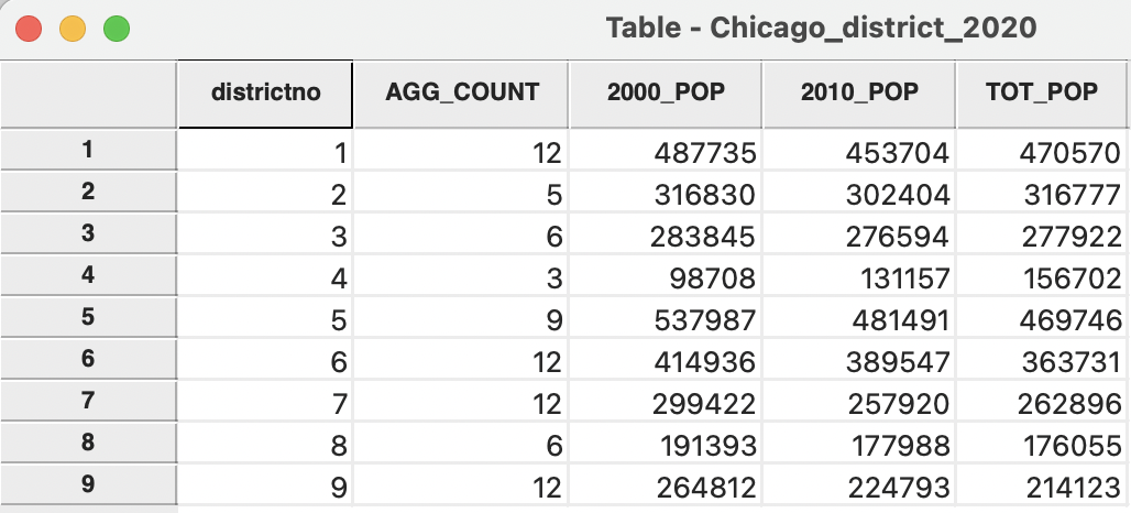
Figure 3.18: Dissolved districts table
3.5.2 Aggregation in table
The same aggregation function is also available as an option for the table, invoked as Table > Aggregate from the menu, or, alternatively, from the list of table options, shown in Figure 2.16. The main difference with the Dissolve function is that the results are only available as a table, without an associated dissolved map.
The dialog requests the same three features and operates in the same way as shown in Figure 3.16.20 The result is saved as a table, which contains the same information as shown in Figure 3.18.