20.4 DBSCAN*
One of the potentially confusing aspects of DBSCAN is the inclusion of so-called Border points in a cluster. The DBSCAN* algorithm, outlined in Campello, Moulavi, and Sander (2013) and further elaborated upon in Campello et al. (2015), does away with the notion of border points, and only considers Core and Noise points.
Similar to the approach in DBSCAN, a Core object is defined with respect to a distance threshold (Eps) as the center of a neighborhood that contains at least Min Points other observations. All non-core objects are classified as Noise (i.e., they do not have any other point within the distance range Eps). Two observations are Epsilon reachable if each is part of the Epsilon-neighborhood of the other. Core points are density-connected when they are part of a chain of Epsilon-reachable points. A cluster is then any largest (i.e., all eligible points are included) subset of density connected pairs. In other words, a cluster consists of a chain of pairs of points that belong to each others Epsilon-neighborhoods.
20.4.1 Mutual Reachability Distance
An alternative perspective on the concept of Epsilon-neighborhoods is to consider the duality between density of points within a given radius and the distance needed to reach a given number of neighbor points. More specifically, the requirement of having k neighbors (Minimum Points - 1) within a given Epsilon distance range can be replaced by considering the k-nearest neighbor distance for a point. The smaller the distance required to reach the k-nearest neighbor, the denser the point distribution will be, and vice versa. In DBSCAN* and HDBSCAN (see Section 20.5), this is called the core distance (\(d_{core}\)) for a given k. The larger the core distance, the less dense is the point distribution around the reference location.
This consideration leads to a new concept of distance between two points A and B, defined as the mutual reachability distance. This is a compromise between the actual inter-point distance, \(d_{AB}\) and the density of the points, reflected in the respective core distances, \(d_{core}(A)\) and \(d_{core}(B)\). Specifically, even though A and B may be close, if they are in low density regions, their inter-point distance will be replaced by the larger of \(d_{core}(A)\) and \(d_{core}(B)\), effectively pushing the points further away from each other. Formally, the mutual reachability distance between A and B is defined as: \[d_{mr}(A,B) = max[d_{core}(A),d_{core}(B),d_{AB}].\] This mutual reachability distance replaces the original distance \(d_{AB}\) in the connectivity graph that forms the basis for the determination of clusters (e.g., a graph like Figure 20.5). Unless A and B are mutual k-nearest neighbors, this effectively replaces the inter-point distances by a core distance.130
In DBSCAN*, the adjusted connectivity graph is reduced to a minimum spanning tree or MST (see Section 3.4) to facilitate the derivation of clusters. Rather than finding a single solution for a given distance range as in DBSCAN, the longest edges in the MST are cut sequentially to provide a solution for each value of inter-point mutual reachability distance. This boils down to finding a cut for smaller and smaller values of the core distance. It yields a hierarchy of clusters for decreasing values of the core distance.
In practice, one starts by applying a cut between two edges that are the furthest apart. This either results in a single point splitting off (a Noise point), or in the single cluster to split into two (two subtrees of the MST). Subsequent cuts are applied for smaller and smaller distances. Decreasing the critical distance is the same as increasing the density of points, referred to as \(\lambda\) in this context (see Section 20.5).
As Campello et al. (2015) show, applying cuts to the MST with decreasing distance (or increasing density) is equivalent to applying cuts to a dendrogram obtained from single linkage hierarchical clustering using the mutual reachability distance as the dissimilarity matrix (hierarchical clustering methods are considered in Volume 2).
DBSCAN* derives a set of flat clusters by applying a cut to the dendrogram associated with a given distance threshold. The main difference with the original DBSCAN is that border points are no longer considered. In addition, the clustering process is visualized by means of a dendrogram. However, in all other respects it is similar in spirit, and it still suffers from the need to select a distance threshold.
20.4.2 Implementation
DBSCAN* is invoked in the same way as DBSCAN, but with DBScan* checked as the Method in the DBScan Clustering Settings dialog (Figure 20.7). All other settings are the same, except that now the Min. Cluster Size option becomes available. However, in practice, this is typically set equal to the Min Points parameter and it is seldom used.
The functionality operates largely the same as for DBSCAN, except that the first result for a given Min Points is a Dendrogram, shown in the right panel of the dialog. Figure 20.10 depicts the dendrogram for the same settings as in Figure 20.9, i.e., with a threshold distance of 50km and 10 minimum points. However, the results are very different. Only two clusters are identified, compared to 7 clusters before. They are visualized by selecting the Save/Show Map button at the bottom of the dialog.
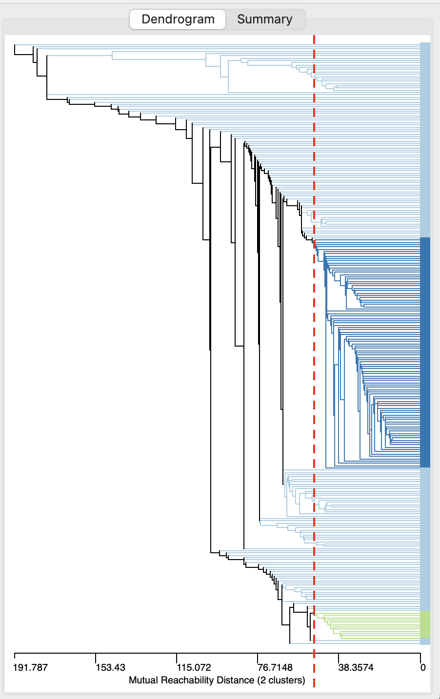
Figure 20.10: DBSCAN-Star Dendrogram, Eps=50, Min Pts=10
The resulting cluster map is shown in Figure 20.11. One cluster is very large, containing 100 observations, the other is small, with only 12 observations. A total of 149 observations are classified as Noise. Relative to the DBSCAN solution in Figure 20.9, the fit declined to a ratio of 0.894.
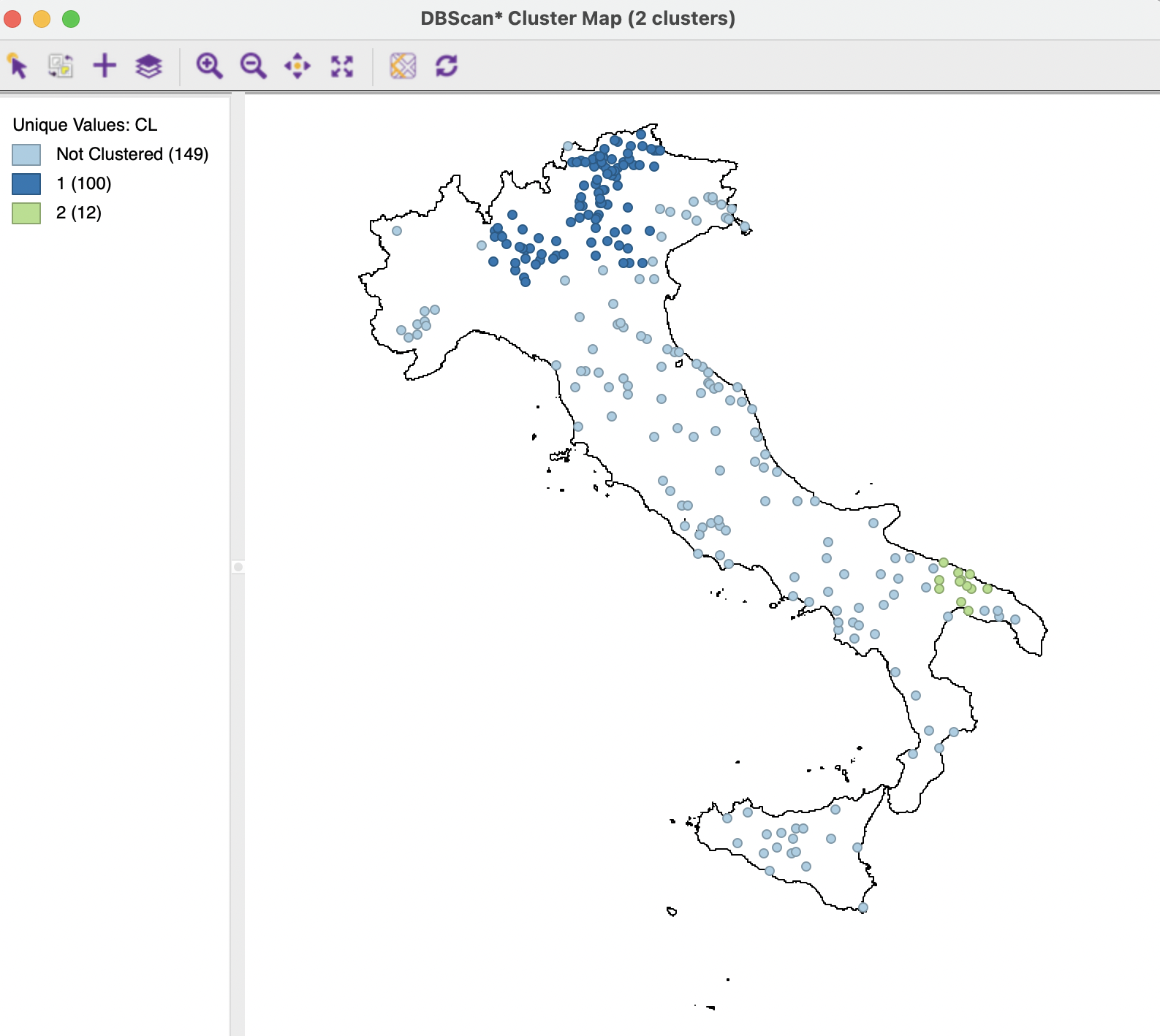
Figure 20.11: DBSCAN-Star Cluster Map, Eps=50, Min Pts=10
20.4.2.1 Exploring the dendrogram
The main advantage of DBSCAN* over DBSCAN is a much more straightforward treatment of Border points (they are all classified as Noise), and an easy visualization of the sensitivity to the threshold distance by means of a dendrogram. Clusters can be explored for different core distances. As long as Min Points (and the minimum cluster size) remains the same, the dendrogram can be used to assess the cluster structure for different threshold distance cut values. This is implemented by moving the cut-off line in the dendrogram. The distance on the horizontal axis is the mutual reachability distance or core distance, and it replaces the original inter-point distances.
For example, in the right-hand panel of Figure 20.12, the dashed red line corresponding to the cut-off distance is moved to the left, to a distance of 73km (also used in Section 11.4.2). The corresponding cluster map is shown in the left-hand panel. The number of clusters has doubled to four, ranging in size from 151 to 11 observations, with 53 unclustered Noise points. The fit ratio decreases to 0.855.
The map may give the impression that seemingly disconnected points are contained in the same cluster. In the example, the points within the red rectangle contain both observations that belong to cluster 1 (dark blue) as well as unclustered points (light blue). This seeming contradiction is due to the fact that the core distance is used in the dendrogram, and not the actual inter-point distance.
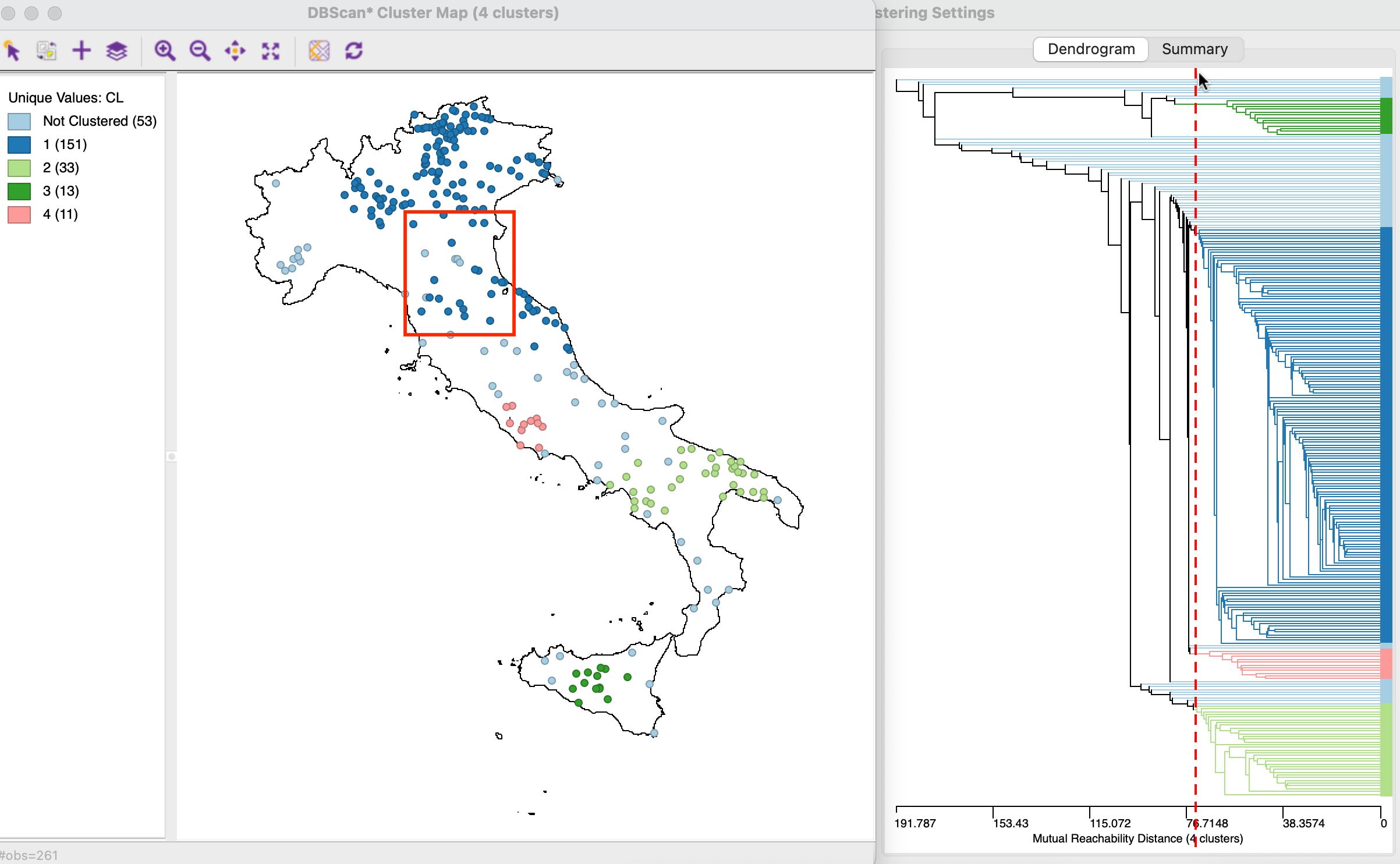
Figure 20.12: Exploring the Dendrogram
The dendrogram needs to be reconstructed for each different value of Min Points, since this critically affects the mutual reachability and core distances.
The main disadvantage of DBSCAN*, just as for DBSCAN, remains that the same fixed threshold distance must be applied to all clusters, yielding a so-called flat cluster. This is remedied by HDBSCAN.
The largest k-nearest neighbor distance will always be larger than the inter-point distance, unless A and B are mutual k-nearest neighbors, in which case \(d_{mr}(A,B) = d_{core}(A) = d_{core}(B) = d_{AB}\).↩︎