10.2 The Concept of Spatial Weights

Spatial weights are a key component in any cross-sectional analysis of spatial dependence. As mentioned in the introduction, they are an essential element in the construction of spatial autocorrelation statistics. In addition, spatial weights provide the means to create spatially explicit variables, such as spatially lagged variables and spatially smoothed rates (see Chapter 12).

Spatial weights are a necessary evil. In principle, one would like to have the data determine the strength of the correlation between any pair of observations. However, with only \(n\) observations in a cross-section, it is impossible to estimate all \((n \times n-1)/2\) pairwise correlations. In this situation, growing the sample, i.e., so-called asymptotic analysis, does not help, since the number of correlation parameters grows with \(n^2\), while the sample only increases linearly. In the literature, this is referred to as the incidental parameter problem.⁶⁷ It has no solution other than imposing some structure that simplifies the problem.

The spatial weights accomplish such a simplification by constraining the number of possible neighbor relations. In addition, the same correlation is imposed for all pairs of observations, but this is only relevant in a discussion of global spatial autocorrelation statistics, which is postponed until Part IV.

There are different criteria that can be used to reduce the number of neighbors for each observation. In this chapter, approaches based on the notion of contiguity are considered, i.e., sharing a common border. In spatial analysis, this is typically based on geographic borders, although as discussed in Chapter 11, the concept is perfectly general.

In the remainder of this section, the concept is introduced more formally first, followed by a brief discussion of the two most common forms, i.e., rook and queen contiguity. This is followed by a treatment of the concept of higher order contiguity and some practical considerations.

10.2.1 Spatial weights matrix

A spatial weights matrix expresses the neighbor structure between the \(n\) observations in a cross-section as a \(n \times n\) matrix \(\mathbf{W}\). For each pair \(i-j\), where \(i\) is the matrix row and \(j\) the matrix column, there is a spatial weight element \(w_{ij}\): \[\begin{equation*} \mathbf{W}=\left[ \begin{matrix} w_{11} & w_{12} & \ldots & w_{1n}\\ w_{21} & w_{22} & \ldots & w_{2n}\\ \vdots & \vdots & \ddots & \vdots\\ w_{n1} & w_{n2} & \ldots & w_{nn} \end{matrix} \right]. \end{equation*}\] The spatial weights \(w_{ij}\) are non-zero when \(i\) and \(j\) are neighbors, and zero otherwise. By convention, the self-neighbor relation is excluded, so that the diagonal elements of \(\mathbf{W}\) are zero, \(w_{ii} = 0\).⁶⁸

To make the concept of a spatial weights matrix more concrete, a spatial layout is used with six polygons, shown in Figure 10.2. Two spatial units are defined as neighbors when they share a common border, i.e., when they are contiguous. For example, in the figure, unit 1 shares a border with units 2, 4 and 5, and hence they are neighbors.

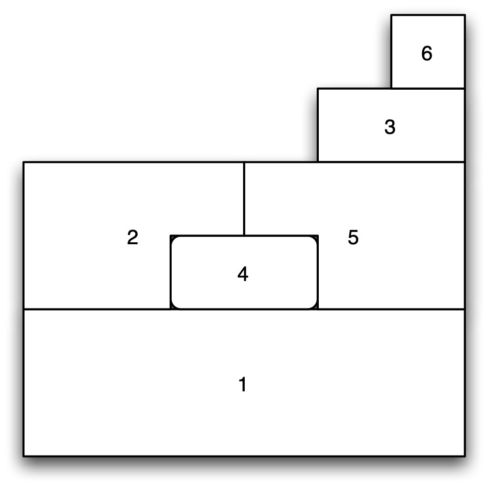
Figure 10.2: Example spatial layout

The same neighbor structure can also be represented in the form of a network or graph, as in Figure 10.3. Here, each spatial unit becomes a node in the network, and the existence of a neighbor relation is represented by an edge or link connecting the respective nodes. Again, node 1 is connected with a link to nodes 2, 4 and 5. It is very important to keep in mind the generality of this network representation, since it applies well beyond purely geographic concepts of contiguity (see Chapter 11).

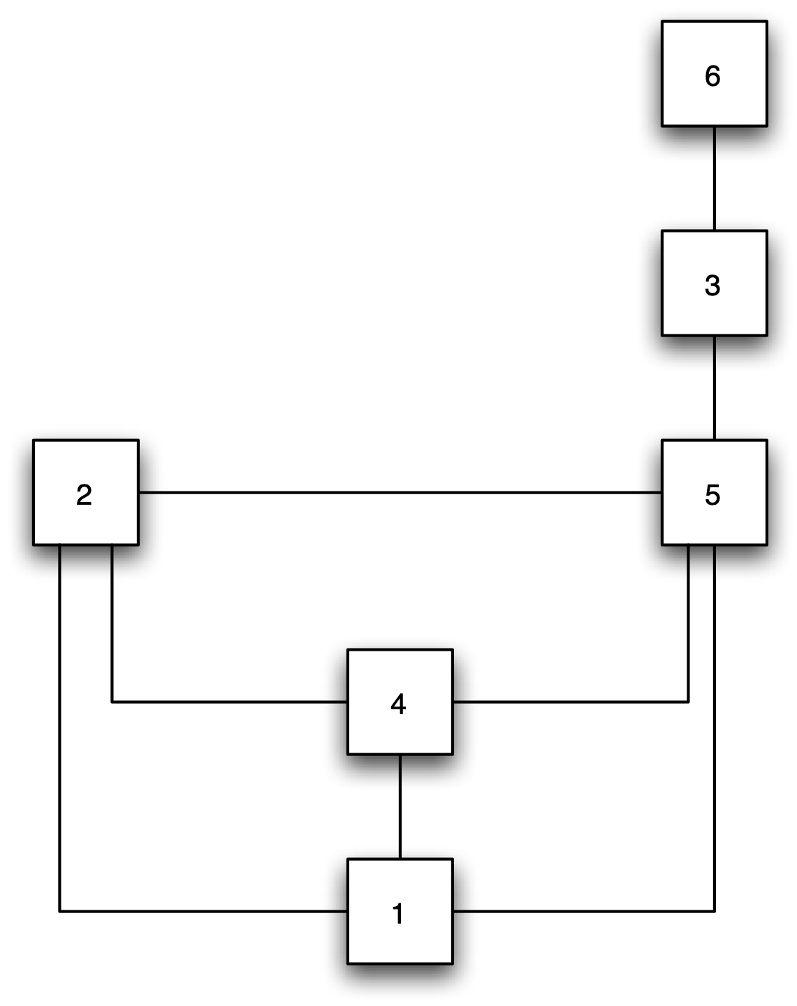
Figure 10.3: Contiguity as a network

In its simplest form, the spatial weights matrix expresses the existence of a neighbor relation in binary form, with weights 1 and 0. For the layout in Figure 10.2, this yields a \(6 \times 6\) matrix: \[\begin{equation}\label{eq:contiguityweights} \mathbf{W} = \left[ \begin{matrix} 0 & 1 & 0 & 1 & 1 & 0\\ 1 & 0 & 0 & 1 & 1 & 0\\ 0 & 0 & 0 & 0 & 1 & 1\\ 1 & 1 & 0 & 0 & 1 & 0\\ 1 & 1 & 1 & 1 & 0 & 0\\ 0 & 0 & 1 & 0 & 0 & 0 \end{matrix} \right]. \end{equation}\] In the first row of this matrix, matching unit 1, the non-zero elements correspond to columns (units) 2, 4 and 5.

In sum, the polygon boundaries in the map layout, the presence of edges in the network, and the non-zero weights in the matrix are all equivalent representations of the topology or spatial arrangement of the data.

While naturally associated with areal units represented as polygons, the notion of contiguity can also be applied in situations where the observations are represented as points, see Section 11.5.1.

Finally, it is important to note that even though it is referred to as a spatial weights matrix, no such matrix is actually used in actual software operations. Spatial weights are typically very sparse matrices, and this sparsity is exploited by using specialized data structures (there is no point in storing lots and lots of zeros).

10.2.1.1 Row-standardizing spatial weights

With a few exceptions, the analyses in GeoDa that employ spatial weights use them in row-standardized form. Row-standardization takes the given weights \(w_{ij}\) (e.g., the binary zero-one weights) and divides them by the row sum: \[\begin{equation*} w_{ij(s)} = w_{ij} / \sum_j w_{ij}. \end{equation*}\] As a result, each row sum of the new matrix equals one. Also, the sum of all weights, \(S_0 = \sum_i \sum_j w_{ij}\), equals \(n\), the total number of observations.⁶⁹

For the layout in Figure 10.2, the matching row-standardized weights matrix is: \[\begin{equation}\label{eq:rowstand} \mathbf{W_s} = \left[ \begin{matrix} 0 & 1/3 & 0 & 1/3 & 1/3 & 0\\ 1/3 & 0 & 0 & 1/3 & 1/3 & 0\\ 0 & 0 & 0 & 0 & 1/2 & 1/2\\ 1/3 & 1/3 & 0 & 0 & 1/3 & 0\\ 1/4 & 1/4 & 1/4 & 1/4 & 0 & 0\\ 0 & 0 & 1 & 0 & 0 & 0 \end{matrix} \right]. \end{equation}\]

Importantly, whereas the original binary weights matrix was symmetric, this is no longer the case with the row-standardized weights. For example, the element in row 1-column 5 equals \(1/3\), whereas the element in row 5-column 1 equals \(1/4\). This has important consequences for some operations in spatial regression analysis, but less so in an exploratory context (but see Section 12.3.1). Also, the weights are no longer equal. In fact, they are inversely related to the number of neighbors. With more neighbors (say, \(k\)), the weight given to each neighboring observation (\(1/k\)) becomes smaller. More importantly, when there is only one neighbor (as in row 6, column 3 in the example), the weights remains 1. This may lead to counter intuitive results when computing spatial transformations, as in Chapter 12.

10.2.2 Types of contiguity

Sharing a common border may seem a straightforward definition of contiguity. However, in practice, it is not always clear what constitutes a border of non-zero length. For example, consider the regular three by three grid layout shown in Figure 10.4

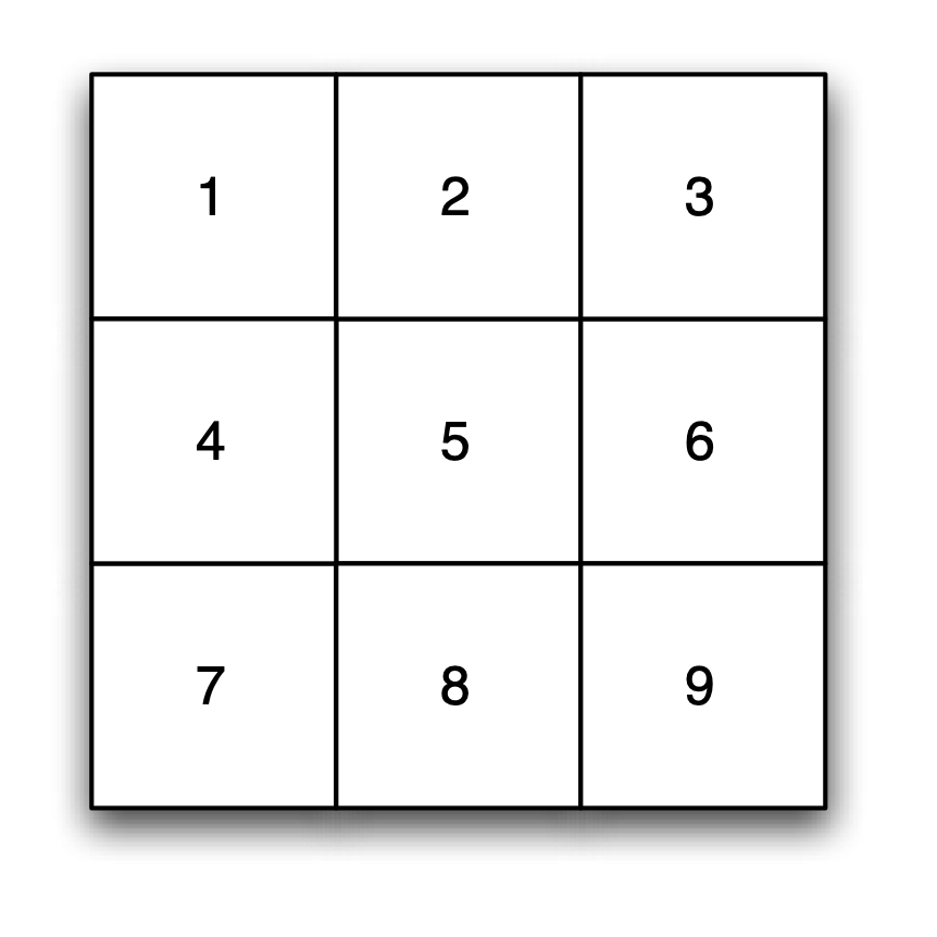
Figure 10.4: Regular grid layout

In this layout, contiguity can be defined in three ways, each yielding a different spatial weights matrix. The three criteria are referred to as rook, bishop and queen, in analogy to the moves allowed by matching pieces on a chess board.

The rook criterion defines neighbors as those cells to the east, west, north and south, yielding four neighbors for each spatial unit that is not on the boundary of the spatial layout. In the example, this yields 2, 4, 6 and 8 as the neighbors of cell 5, as shown in Figure 10.5.

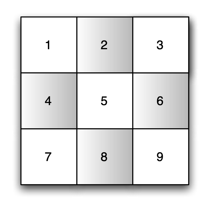
Figure 10.5: Rook contiguity

The matching binary contiguity weights matrix for the nine spatial units is then the \(9 \times 9\) matrix: \[\begin{equation} \mathbf{W} = \left[ \begin{matrix} 0 & 1 & 0 & 1 & 0 & 0 & 0 & 0 & 0\\ 1 & 0 & 1 & 0 & 1 & 0 & 0 & 0 & 0\\ 0 & 1 & 0 & 0 & 0 & 1 & 0 & 0 & 0\\ 1 & 0 & 0 & 0 & 1 & 0 & 1 & 0 & 0\\ 0 & 1 & 0 & 1 & 0 & 1 & 0 & 1 & 0\\ 0 & 0 & 1 & 0 & 1 & 0 & 0 & 0 & 1\\ 0 & 0 & 0 & 1 & 0 & 0 & 0 & 1 & 0\\ 0 & 0 & 0 & 0 & 1 & 0 & 1 & 0 & 1\\ 0 & 0 & 0 & 0 & 0 & 1 & 0 & 1 & 0 \end{matrix} \right]. \end{equation}\] The structure of the weights matrix is characterized by a band of ones. In addition, there is a strong effect of boundary units in this small data set. Internal units have four neighbors, but corner units only have two, and the other boundary units only have three.

A second criterion to define contiguity, less frequently used, is based on common vertices (corners) as the convention to identify neighbors. This is referred to as bishop contiguity. Due to its lack of adoption in practice, it is not further considered here.

Finally, the queen criterion combines rook and bishop. As a result, neighbors share either a common edge or a common vertex. This yields eight neighbors for the non-boundary units. For example, as shown in Figure 10.6, the central cell 5 has all the other cells being neighbors.

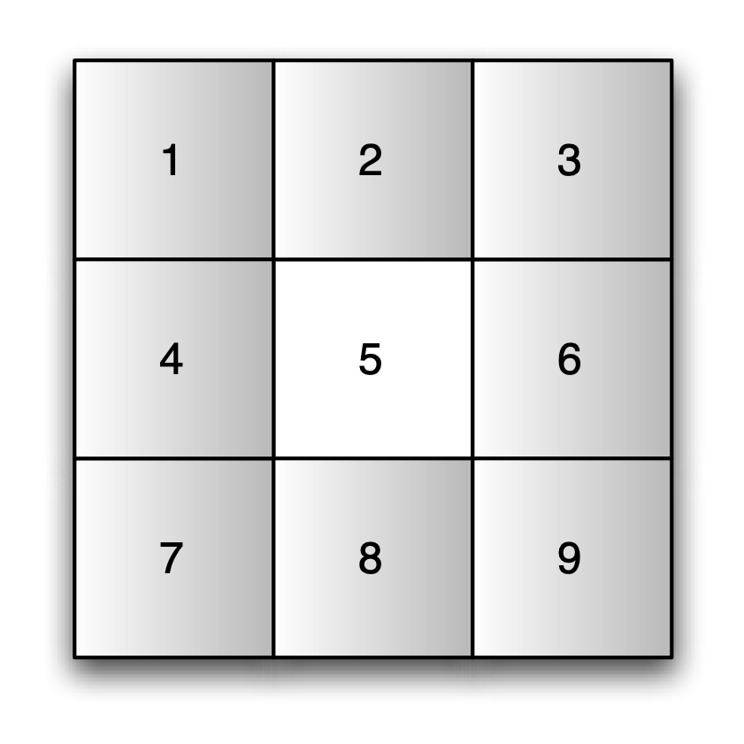
Figure 10.6: Queen contiguity

The matching \(9 \times 9\) binary contiguity matrix is much denser than before: \[ \mathbf{W} = \left[ \begin{matrix} 0 & 1 & 0 & 1 & 1 & 0 & 0 & 0 & 0\\ 1 & 0 & 1 & 1 & 1 & 1 & 0 & 0 & 0\\ 0 & 1 & 0 & 0 & 1 & 1 & 0 & 0 & 0\\ 1 & 1 & 0 & 0 & 1 & 0 & 1 & 1 & 0\\ 1 & 1 & 1 & 1 & 0 & 1 & 1 & 1 & 1\\ 0 & 1 & 1 & 0 & 1 & 0 & 0 & 1 & 1\\ 0 & 0 & 0 & 1 & 1 & 0 & 0 & 1 & 0\\ 0&0&0&1&1 & 1 & 1 & 0 & 1\\ 0&0&0&0&1&1&0&1&0 \end{matrix} \right] \]

Now, the corner cells have three neighbors, and the other boundary cells have five.

The concepts of rook and queen contiguity can easily be extended to other regular tessellations, such as hexagons.⁷⁰ In addition, they apply to irregular lattice layouts as well. In this context, rook neighbors are those spatial units that share a common edge, and queen neighbors those that share either a common edge or a common vertex. As a result, spatial weights based on the queen criterion will always have at least as many neighbors as a corresponding rook-based weights matrix.

In practice, whether a common segment is categorized as a point (vertex) or line segment (edge) depends on the precision of the geocoding in a GIS. Due to generalization (a process of simplifying the detail in a spatial layer), some small line segments may be represented as points in one GIS and not in another. In addition, similar quirks in the representation of polygon boundaries may result in (very) small empty spaces between them. In a naive approach to defining common boundaries, such instances would fail to identify neighbors. Therefore, some tolerance may be required to make the weights creation robust to such characteristics.

10.2.3 Higher-Order contiguity

So far, the focus has been on the notion of a direct neighbor, or, more precisely, a first order neighbor. The concept of contiguity can be generalized to allow for higher order neighbors, similar to the time series context, where a time shift can pertain to multiple periods.

A higher order neighbor is defined in a recursive fashion, as a first order neighbor to a lower order neighbor. More formally, \(j\) is a neighbor of order \(k\) to \(i\) if:

• \(j\) is a first order neighbor to \(h\),
• \(h\) and \(i\) are neighbors of order \(k - 1\), and
• \(j\) is not already a lower order neighbor to \(i\).

Using this logic, candidates to be a second order neighbor would be any first order neighbor to another observation that is already a first order neighbor. However, this would be limited to only those locations that are not already first order neighbors. Parenthetically, it should be noted that the concept of higher order contiguity is similar to the notion of reachability in social networks (e.g., Newman 2018).

In the layout shown in Figure 10.7, cells 4 and 3 are highlighted. Cell 4 has three first order neighbors, immediately surrounding it: 1, 2 and 5. Cell 3 is a first order neighbor to 5, hence 3 is a second order neighbor to 4.

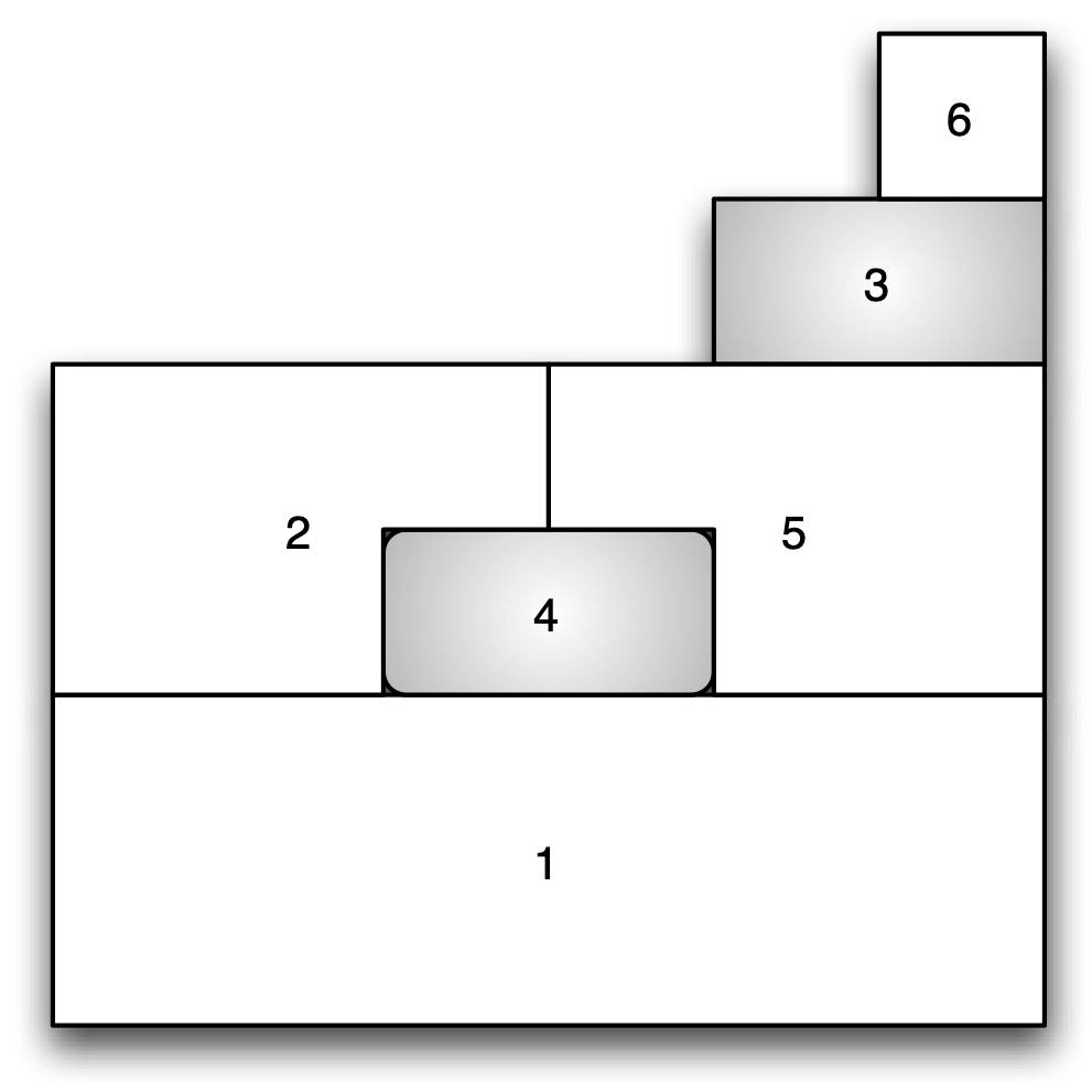
Figure 10.7: Second order contiguity

In the graph representation of the contiguity structure in Figure 10.8, second order contiguity corresponds to of a path of length 2 from node 4 to node 3, illustrated by the dashed lines. This path requires the traversal of two edges in the graph, [4-5] and [5-3], and is thus of length 2. As it turns out, the number of edges separating a pair of nodes corresponds to the order of contiguity.

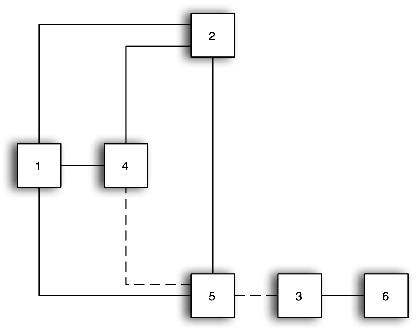
Figure 10.8: Higher order contiguity as multiple steps in the graph

As such, identifying paths of length 2 between nodes is not sufficient to find the correct second order neighbors, since it does not preclude redundant or circular paths. For example, a closer examination of Figure 10.8 reveals that 1 and 5 can be reached in two steps from 4 as well (e.g., 4-1-2, 4-5-1). In fact, multiple paths of length 2 can exist between two nodes (e.g., 4-1-2 and 4-5-2).

These paths illustrate the complexity of the problem of finding higher order neighbors. For example, nodes 2 and 5 cannot be both first order and second order neighbors of node 4, so a strict application of the graph-theoretical approach is not sufficient in the spatial weights case. Ways must be found to eliminate these redundant paths in order to yield the proper second order neighbor, node 3.

10.2.3.1 Circular and redundant paths

The problem of circular and redundant paths was pointed out early on by Blommestein (1985), in the context of the specification of spatial autoregressive models. For such models, the inclusion of the same observation as a neighbor at different orders of contiguity (e.g., both a first and a second order neighbor) constitutes a so-called identification problem (it is impossible to tell certain parameters apart). An efficient algorithm to remove such redundancies is developed by Anselin and Smirnov (1996), based on shortest paths in the network structure.

However, in an exploratory context, it may be useful to include lower order neighbors in order to mimic the effect of expanding bands of neighbors, similar to an expanding distance band (see Section 11.3.1). GeoDa includes both concepts of higher order weights (Section 10.3.4).

10.2.4 Practical considerations

In practice, the construction of the spatial weights from the geometry of the data cannot be done by visual inspection or manual calculation, except in the most trivial of situations. Specialized software is needed to compute distances between points from their coordinates or to derive the presence of common borders from the boundary information for polygons.

To assess whether two polygons are contiguous is quite demanding. This requires the use of explicit spatial data structures to deal with the location and arrangement of the polygons, a functionality that is lacking in most econometric and statistical software. The specialized spatial data representation that differentiates a GIS from a standard data base system, and especially the use of a spatial index are crucial in this respect.

Many commonly used spatial data structures are in a so-called spaghetti representation. While this approach is more efficient for rapid rendering of maps, it lacks indexing and topology. It is popular in many cartographic packages and map-oriented GIS. A well known example is ESRI’s shape file format.

GeoDa uses its own internal data structure to represent polygons loaded from different sources (files as well as spatial data bases), so that it can take advantage of spatial indexing to optimize the generation of the weights information.

It is important to keep in mind that the spatial weights are critically dependent on the quality of the spatial data source (GIS) from which they are constructed. Problems with the topology in the GIS (e.g., slivers) will result in inaccuracies for the neighbor relations included in the spatial weights. In practice, it is essential to check the characteristics of the weights for any evidence of problems. When problems are detected, the solution is to go back to the GIS and fix or clean the topology of the data set. Editing of spatial layers is not implemented in GeoDa, but this is a routine operation in most GIS software.

---

67. See Lancaster (2000) for a technical review.↩︎

68. An exception to this rule are the diagonal elements in kernel-based weights, which are considered in Chapter 12.↩︎

69. Strictly speaking, this is only correct in the absence of so-called isolates, i.e., observations without neighbors. With \(q\) isolates, the sum \(S_0 = n - q\). See Section 11.4.2.↩︎

70. In the literature pertaining to cellular automata, counterparts to the rook and queen contiguity are the so-called von Neumann and Moore neighborhoods. The main difference is that here, the central cell is not included in the neighborhood concept, whereas it is in cellular automata.↩︎