17.3 Local Geary

The Local Geary statistic, first outlined in Anselin (1995), and further elaborated upon in Anselin (2019a), is a Local Indicator of Spatial Association (LISA) based on a measure of attribute similarity that differs from the cross-product. As in its global counterpart, the focus is on squared differences, or, rather, dissimilarity. In other words, small values of the statistics suggest positive spatial autocorrelation, whereas large values suggest negative spatial autocorrelation.

As introduced in Section 13.4.3.2, the Geary c statistic of global spatial autocorrelation (Geary 1954) takes on the following form: \[c = \frac{\sum_i \sum_j w_{ij}(x_i - x_j)^2/2S_0}{\sum_i (x_i - \bar{x})^2 / (n-1)},\] with \(S_0 = \sum_i \sum_j w_{ij}\), and where the \(x\) in the numerator do not need to be in standardized form, due to the squared difference. The statistic has a mean value of 1 under the null hypothesis of spatial randomness. Significant values less than 1 indicate positive spatial autocorrelation and values larger than 1 negative spatial autocorrelation.

After controlling for the parts in the expression that do not change with \(i\), a local version of the statistic can be found as (for technical details, see Anselin 1995): \[c_i = \sum_j w_{ij}(x_i - x_j)^2,\] or as: \[c_i = (1/m_2) \sum_j w_{ij}(x_i - x_j)^2,\] with \(m_2 = \sum z_i^2 / n\). Again, because of the squared difference, there is no need to standardize \(x\).

The sum over all the local statistics is: \[\sum_i c_i = n [ \sum_i \sum_j w_{ij} (x_i - x_j)^2 / \sum_i z_i^2].\] In comparison, Geary’s global c statistic can be reformulated as: \[c = [(n-1)/2S_0] [ \sum_i \sum_j w_{ij} (x_i - x_j)^2 / \sum_i z_i^2].\] This establishes the connection between the local and the global as: \[\sum_i c_i = 2nS_0/(n - 1) c.\] Hence, the Local Geary is a LISA statistic in the sense established in Section 16.2.

Closer examination reveals that the Local Geary statistic consists of a weighted sum of the squared distance in attribute space for the geographical neighbors of observation \(i\). Since there is no cross-product involved, there is no direct relation to linear similarity. In other words, since the Local Geary uses a different criterion of attribute similarity, it may detect patterns that escape the Local Moran, and vice versa.

As for the Local Moran, analytical inference is based on an approximation and generally not very reliable. Instead, the same conditional permutation procedure as for the Local Moran is implemented. The results are interpreted in the same way, with the caveat regarding the p-values and the notion of significance.

17.3.1 Implementation

the Local Geary can be invoked from the Cluster Maps toolbar icon, as the first item in the fourth block in the drop down list. Alternatively, it can be started from the main menu, as Space > Univariate Local Geary.

The subsequent step is the same as before, bringing up the Variable Settings dialog that contains the names of the available variables as well as the spatial weights. Everything operates in the same way for all local statistics.

The final dialog offers window options. In the case of the local Geary, there is no Moran scatter plot option, but only the Significance Map and the Cluster Map. The default is that only the latter is checked, as before.

With the variable p_PHA(2010) (or p_PHA10), queen contiguity (oaxaca_q) and 99,999 permutations, the significance map and cluster map for the Local Geary statistic, using p < 0.05 are shown in Figure 17.11.

The significance map uses the same conventions as before, but the cluster map is different. There are four different types of associations, three for clusters and one for spatial outliers. The classification is further elaborated upon in Section 17.3.2. Comparison with the results for a Local Moran statistic is considered in Section 17.3.3.

Overall, there are 108 locations indicating positive spatial autocorrelation, contrasted with only 16 locations for negative spatial autocorrelation.

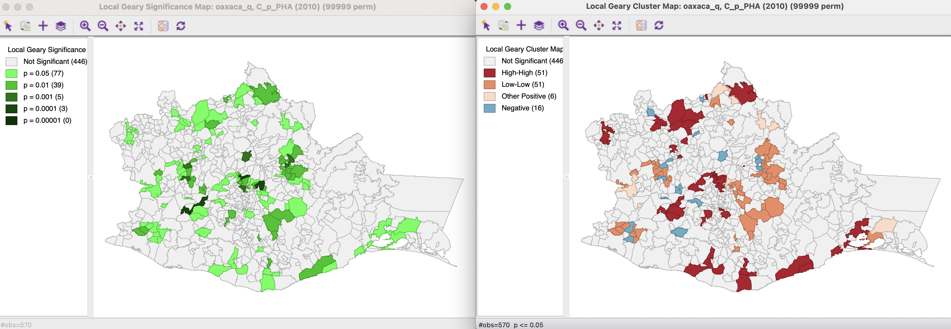
Figure 17.11: Local Geary significance and cluster maps

All the options operate the same for all local statistics, including the randomization setting, the selection of significance levels, the selection of cores and neighbors, the conditional map option, as well as the standard operations of setting the selection shape and saving the image.

17.3.1.1 Saving the results

The Save Results option again includes the possibility to save the statistic itself (Geary_I), the cluster indication (Geary_CL) and the significance (Geary_P). The code for the cluster classification for the Local Geary is 0 for not significant, 1 for a High-High cluster core, 2 for a Low-Low cluster core, 3 for other positive spatial autocorrelation, and 4 for negative spatial autocorrelation.

17.3.2 Clusters and spatial outliers

The interpretation of significant locations in terms of the type of association is not as straightforward for the Local Geary as it was for the Local Moran. In essence, this is because the attribute similarity is a squared difference and not a cross-product, and thus has no direct correspondence with the slope in a scatter plot. Nevertheless, the linking capability within GeoDa can be exploited to accomplish classification, albeit an incomplete one.

The locations identified as significant and with the Local Geary statistic smaller than its mean, suggest positive spatial autocorrelation (small differences imply similarity). Those observations that can be classified in the upper-right or lower-left quadrants of a matching Moran scatter plot, are identified as High-High or Low-Low. However, given that the squared difference can cross the mean, there may be observations for which such a classification is not possible. Those are referred to as other positive spatial autocorrelation.

For negative spatial autocorrelation (large values imply dissimilarity), it is not possible to assess whether the association is between High-Low or Low-High outliers, since the squaring of the differences removes the sign.

This is illustrated in Figures 17.12 through 17.15.

Figure 17.12 shows the case where significant local positive spatial autocorrelation (small Local Geary) corresponds with points in the upper right quadrant of the Moran scatter plot. This matches the concept of High-High clusters introduced before. The corresponding locations are labeled as such in the Local Geary cluster map.

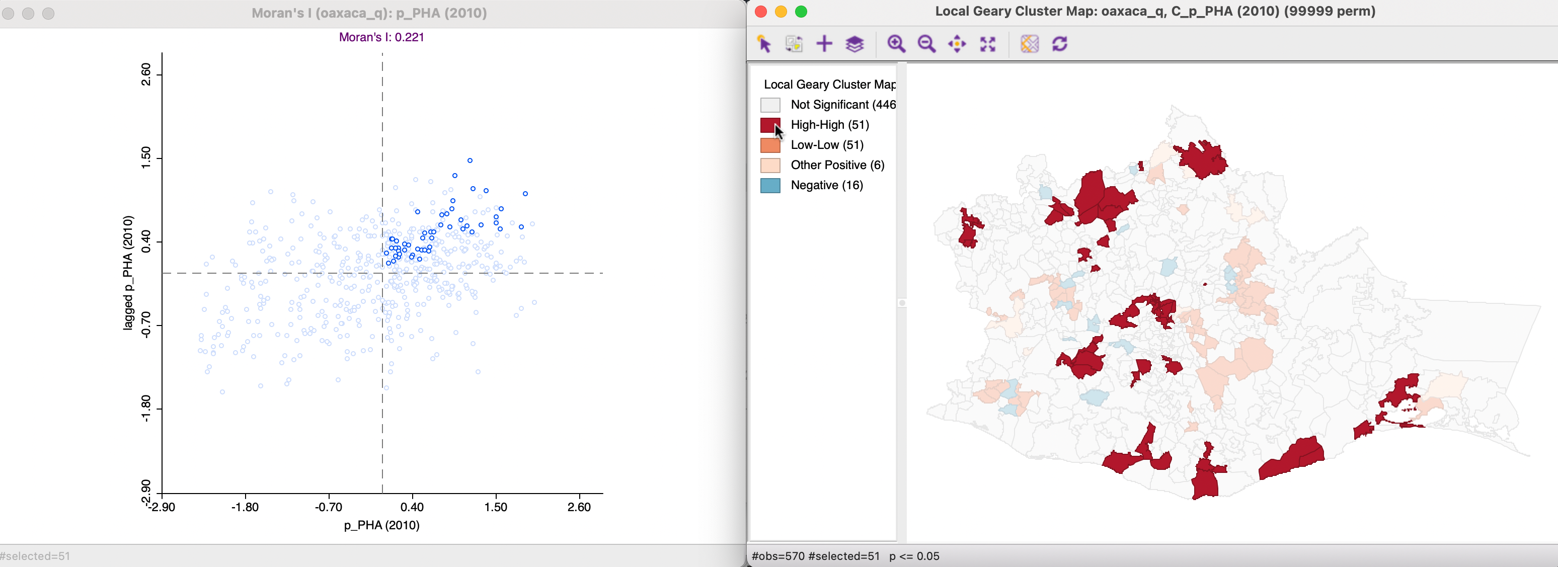
Figure 17.12: Local Geary - High-High clusters

The case where significant local positive spatial autocorrelation corresponds with points in the lower right quadrant of the Moran scatter plot is illustrated in Figure 17.13. This matches the concept of Low-Low clusters, with the matching observations classified as such in the cluster map.

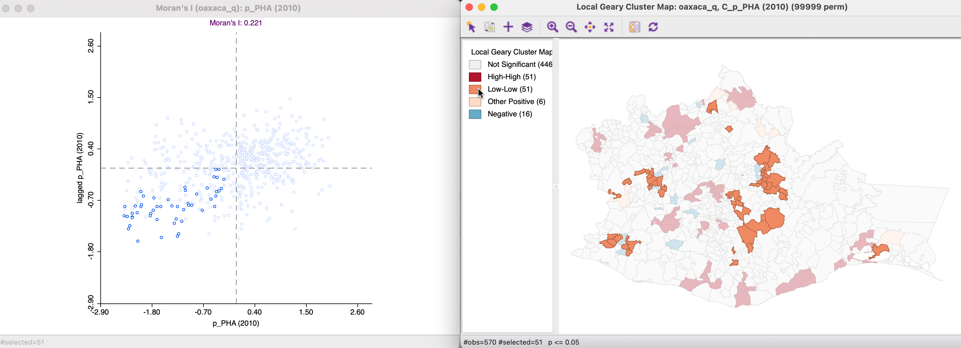
Figure 17.13: Local Geary - Low-Low clusters

The third case of significant positive spatial autocorrelation is illustrated in Figure 17.14. There are six observations for which the Moran scatter plot points appear in the lower right and upper left quadrants, suggesting a mismatch between the cross-product and squared difference attribute measures. Those locations are classified as Other Positive in the cluster map.

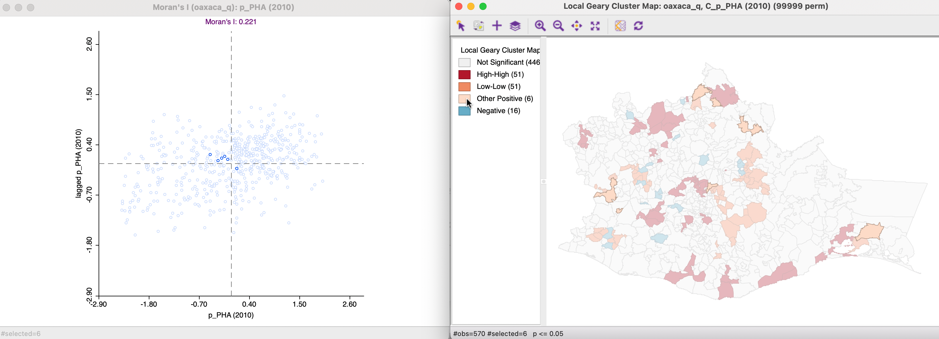
Figure 17.14: Local Geary - Other clusters

Finally, observations with significant negative spatial autocorrelation (large Local Geary) cannot be classified by type of spatial outlier. They are labeled as Negative in the cluster map, as shown in Figure 17.15. All but one of these can also be found in the negative spatial autocorrelation quadrants of the Moran scatter plot, but one is in the lower left quadrant, again suggesting a mismatch between the cross-product and squared difference.

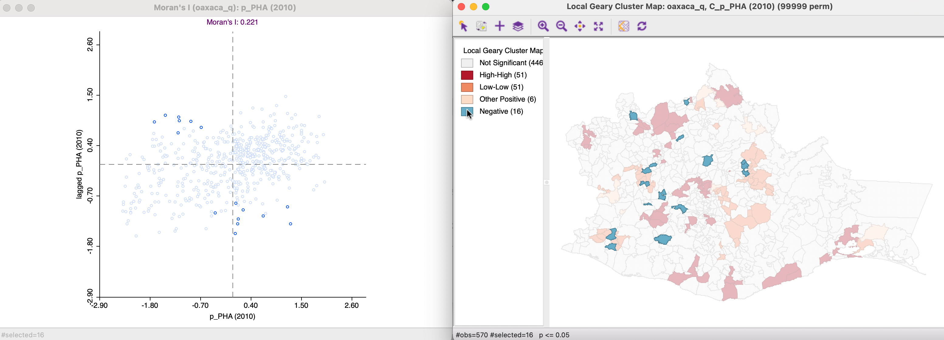
Figure 17.15: Local Geary -spatial outliers

17.3.3 Comparing Local Geary and Local Moran

To gain further insight into the (subtle) difference between the measures of attribute (dis)similarity for the Local Moran and Local Geary statistics, the indications of clusters and spatial outliers obtained by each are considered more closely in what follows. Of course, the findings are not general, and pertain only to the empirical illustration considered here. However, it is useful to carry out such a comparison, especially when interest lies in potential nonlinear associations, which the Local Moran is not able to capture.

Overall, the Local Geary cluster map identifies somewhat more significant locations, yielding 124 such observations relative to 117 for the Local Moran (at p < 0.05), as shown in Figure 17.16.

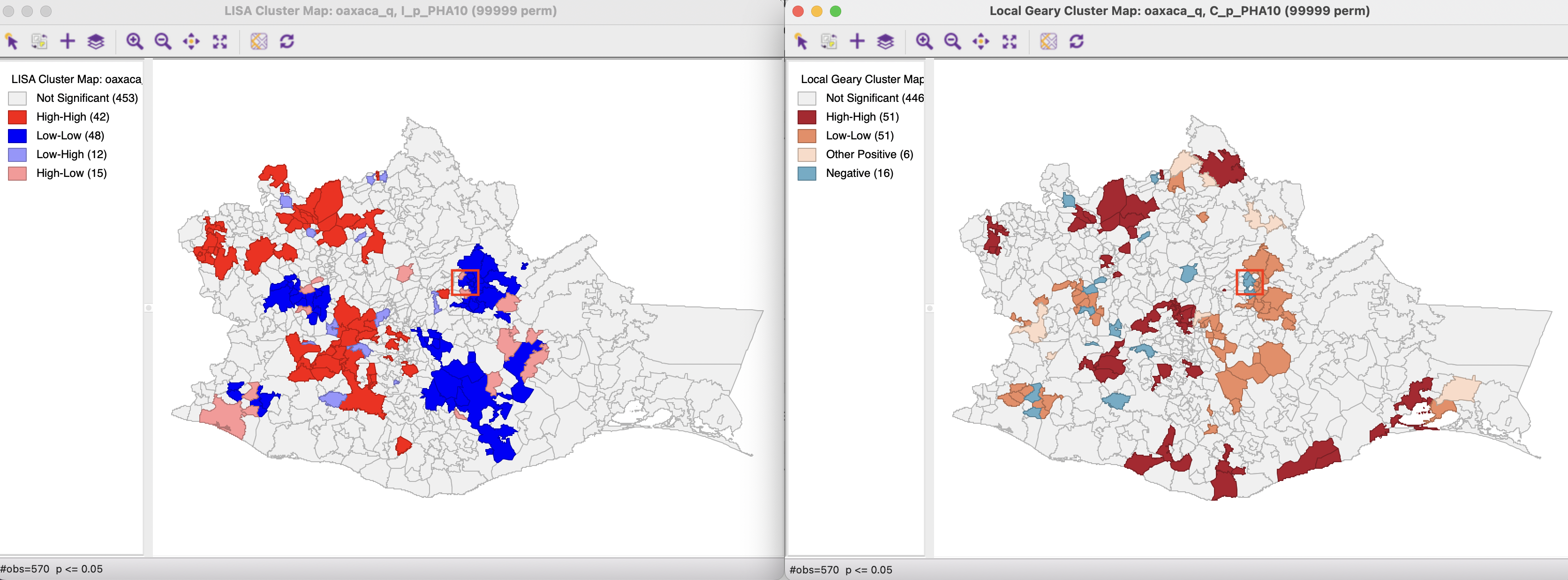
Figure 17.16: Local Geary and Local Moran cluster maps

17.3.3.1 Clusters

Figure 17.17 identifies the matches for the 51 High-High cluster locations in the Local Geary cluster map (on the right) in the Local Moran cluster map (on the left). Only 16 of the 42 Local Moran High-High cluster locations belong to the set identified for the Local Geary, but there are no mismatches in the sense of Low-Low clusters identified. Instead, the non-matches are all not significant for the Local Moran, indicated by their grey color in the map. Similarly, the significant High-High locations in the Local Moran cluster map that are not identified with Local Geary are not significant in the latter (not shown).

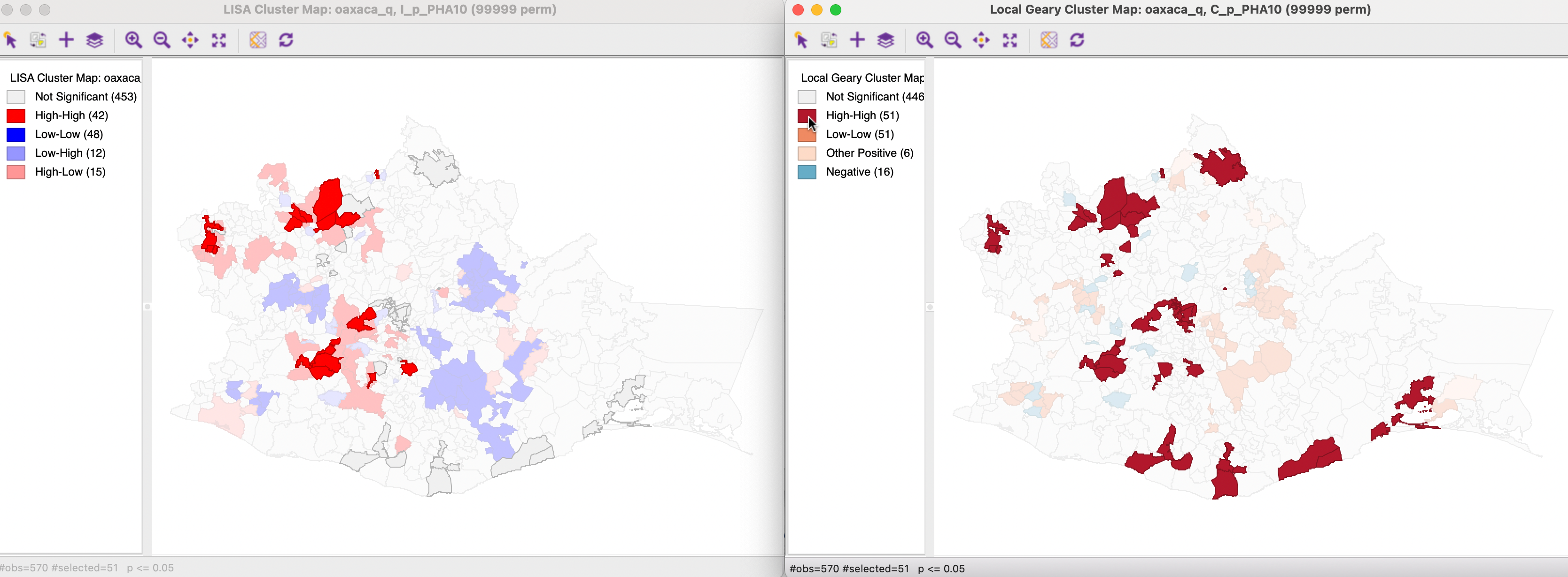
Figure 17.17: Local Geary and Local Moran - High-High clusters

As shown in Figure 17.18, only a subset of the 48 Low-Low clusters for the Local Moran correspond to the 51 such clusters identified by the Local Geary. The other locations are not significant. However, in the reverse order, there is one exception. One of the locations given as a Low-Low cluster by the Local Moran is identified as a spatial outlier (negative) by the Local Geary. The location in question is highlighted in a red rectangle in Figure 17.16. The others are again not significant for Local Geary.

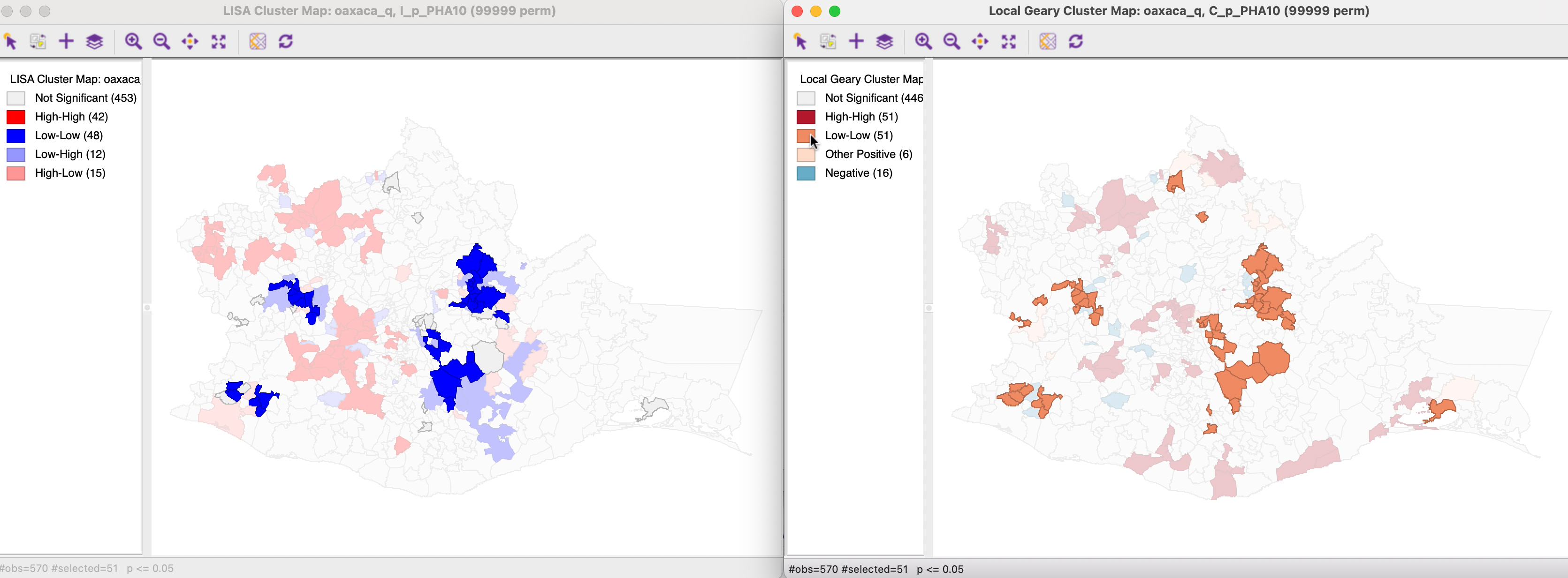
Figure 17.18: Local Geary and Local Moran - Low-Low clusters

Finally, the six other spatial clusters identified in the Local Geary cluster map correspond to non-significant locations for the Local Moran, as shown in Figure 17.19.

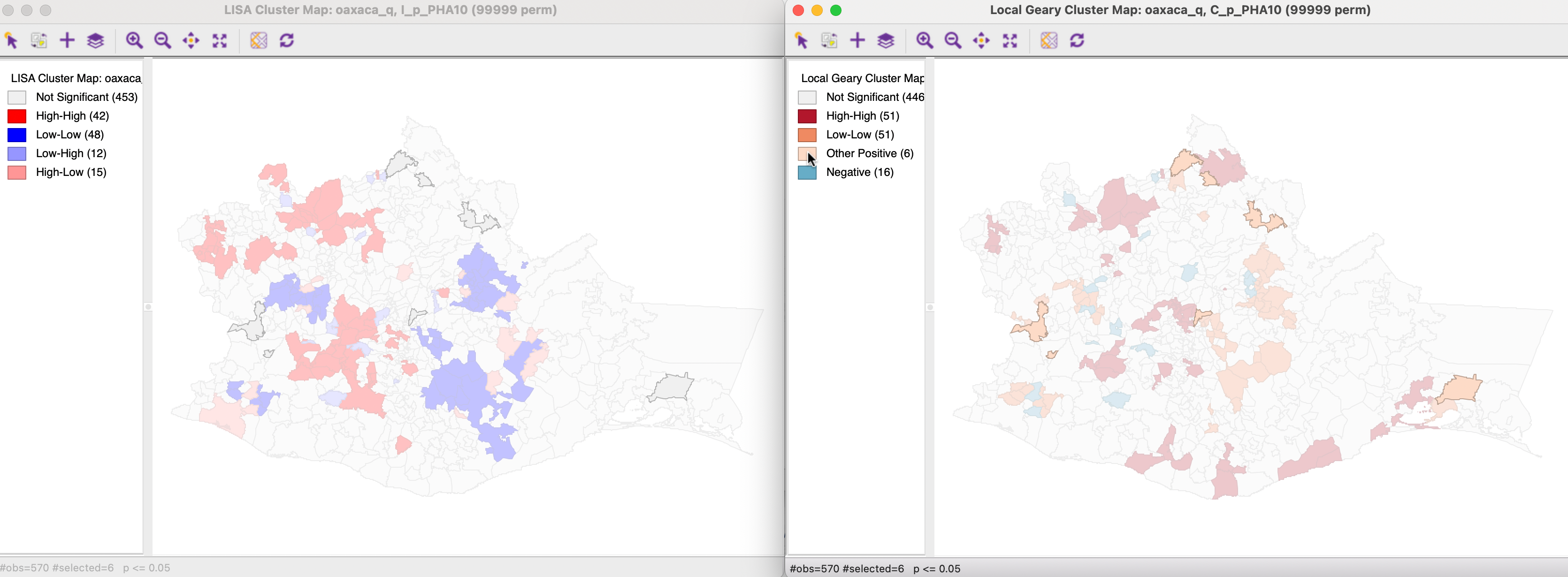
Figure 17.19: Local Geary and Local Moran - Other positive clusters

A careful consideration of the differences and similarities between the identified cluster locations for the two local statistics sheds light on the extent to which the association may be nonlinear. This should be followed by an in-depth inspection of the actual statistics and associated attribute values.

17.3.3.2 Spatial outliers

The Local Geary cluster map indicates 16 locations with significant negative spatial autocorrelation, compared to 27 such outliers for Local Moran. As shown in Figure 17.20, all but one of the spatial outliers for Local Geary match outliers for Local Moran. The same location mentioned earlier is part of a Low-Low cluster for the Local Moran, highlighted by the red rectangle in the maps.

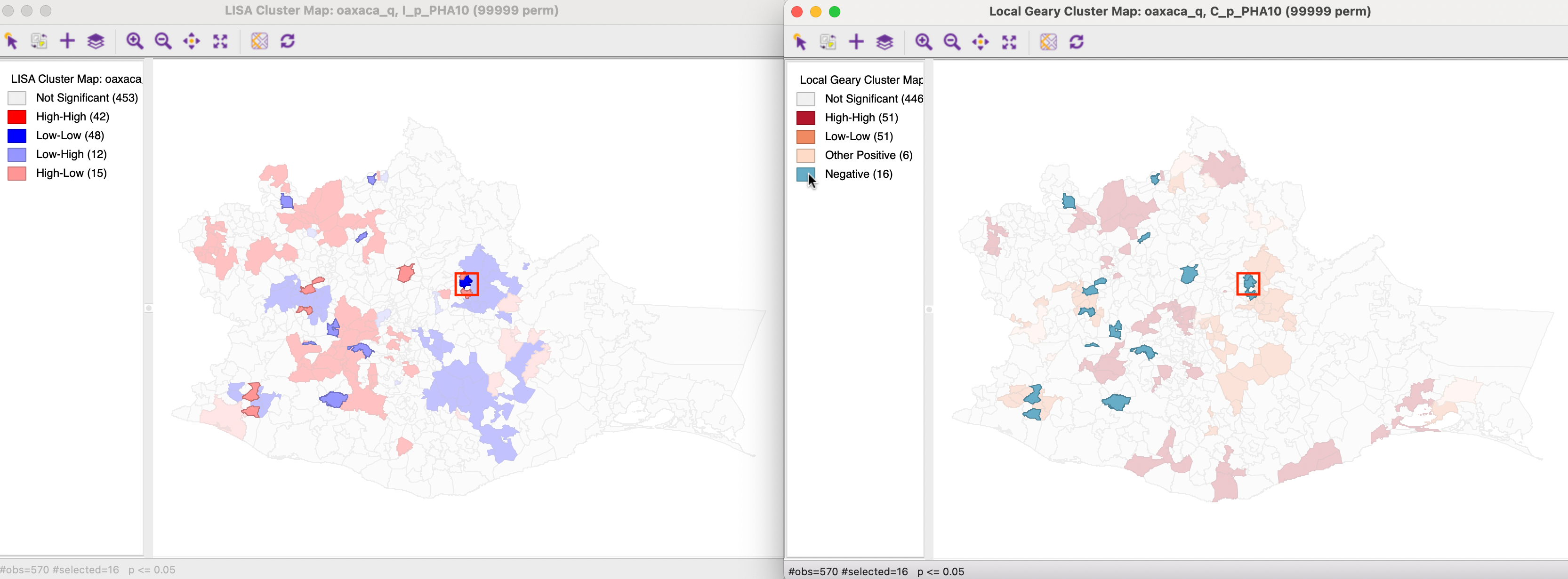
Figure 17.20: Local Geary and Local Moran - spatial outliers

As Figure 17.21 illustrates, the spatial outliers in the Local Moran cluster map all match such outliers for Local Geary or are not significant in the Local Geary cluster map, indicated by the 11 grey polygons.

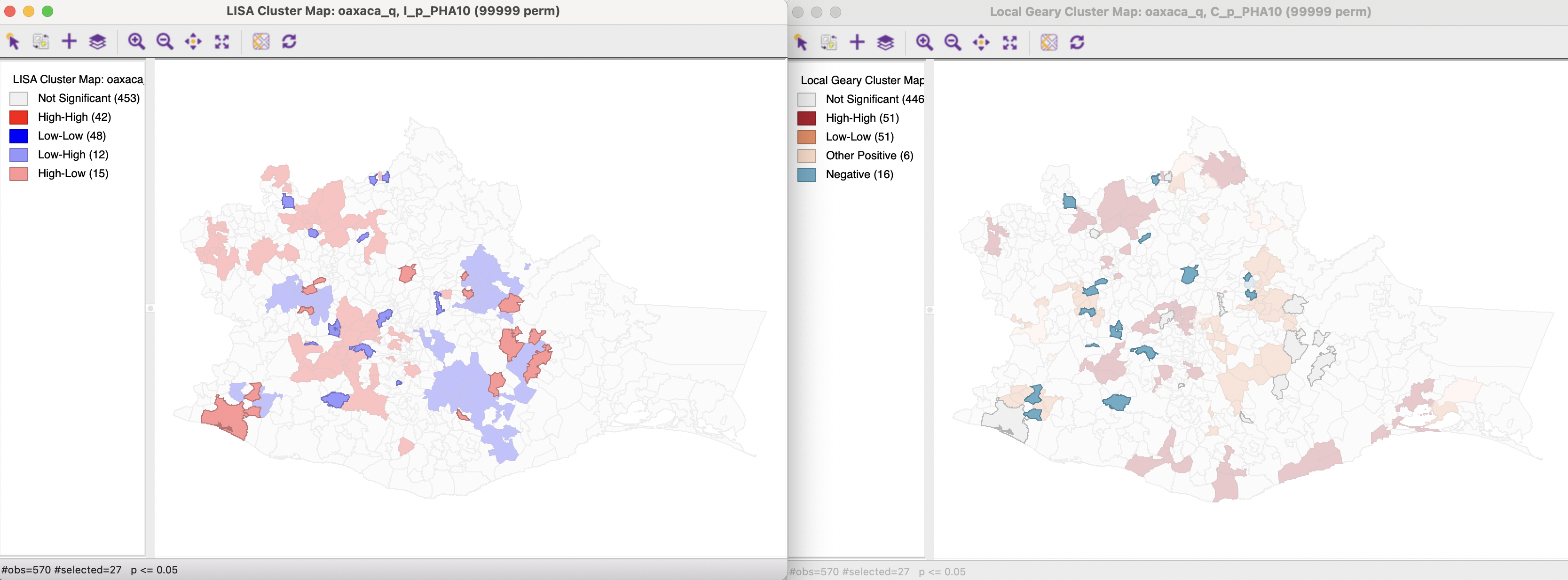
Figure 17.21: Local Moran and Local Geary - spatial outliers