2.3 Creating Spatial Layers

In addition to loading spatial layers from existing files or data base sources, new spatial layers can be created as well. This is implemented through the Tools functionality.

It is invoked from the menu as Tools > Shape, or, alternatively, from the Tools icon on the toolbar, the right-most icon in Figure 2.1. Two different operations are supported: one is to turn X-Y coordinates from a table into a point layer, Tools > Shape > Points from Table, the other creates a rectangular shape of grid cells,Tools > Shape > Create Grid.

2.3.1 Point layers from coordinates

Point layers are created from two variables contained in a data table that can serve as X and Y coordinates. This is illustrated with the file Chicago_2020_carjackings.csv, downloaded from the GeoDaCenter sample data collection. This file contains the same information as Chicago Carjacking in the Sample Data tab, but is a simple comma separated text file.

Once loaded, the contents of the data table are shown in a spreadsheet-like format, as illustrated in Figure 2.9. In the example, the latitude and longitude of the point locations (in decimal degrees) are included as the two last columns in the table. Even though these variables are commonly referred to as lat-lon, latitude is actually the vertical dimension (Y), while longitude is the horizontal dimension (X).

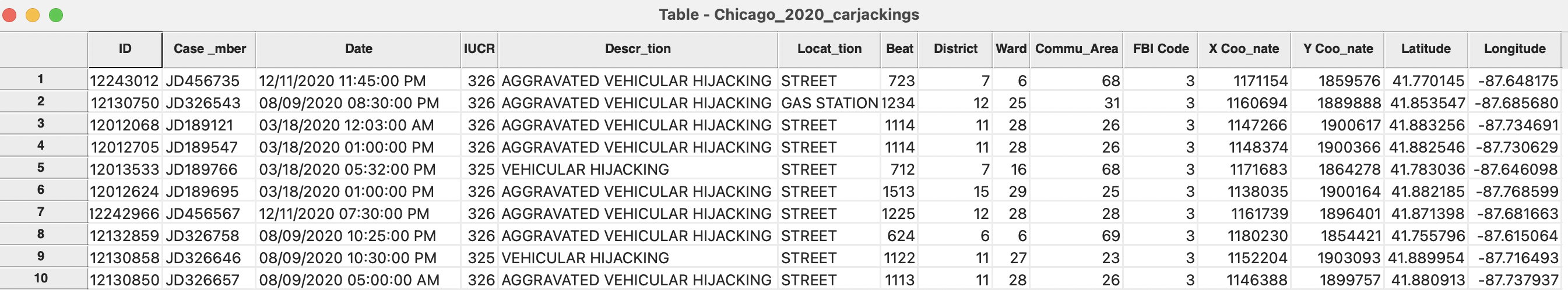
Figure 2.9: Coordinate variables in data table

The Tools > Shape > Points from Table command opens up a dialog that lists all numerical variables contained in the data table. In the example, shown in Figure 2.10, the variables to be selected are Longitude and Latitude.

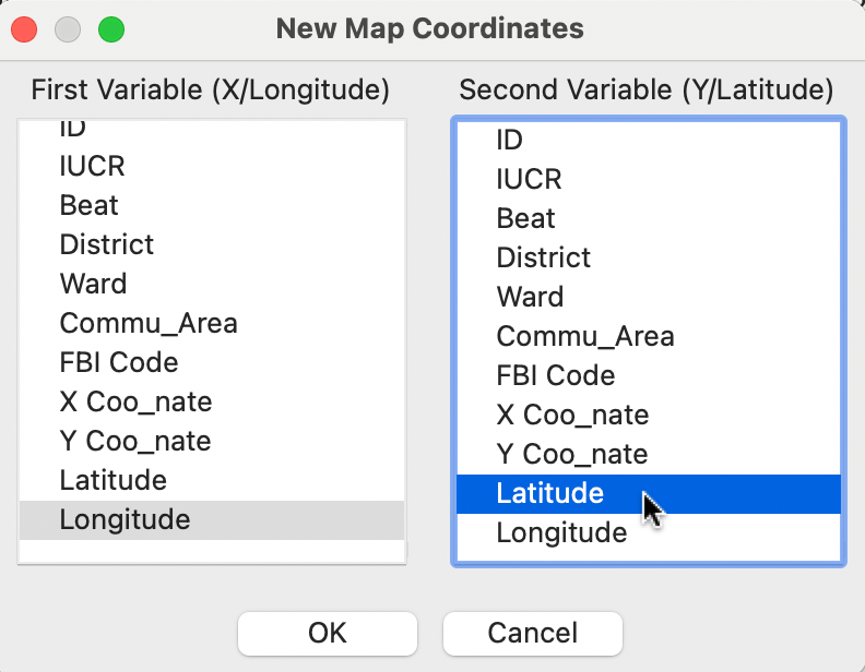
Figure 2.10: Specifying the point coordinates

After specifying the coordinate variables and clicking on OK, a point map appears, as in Figure 2.11.

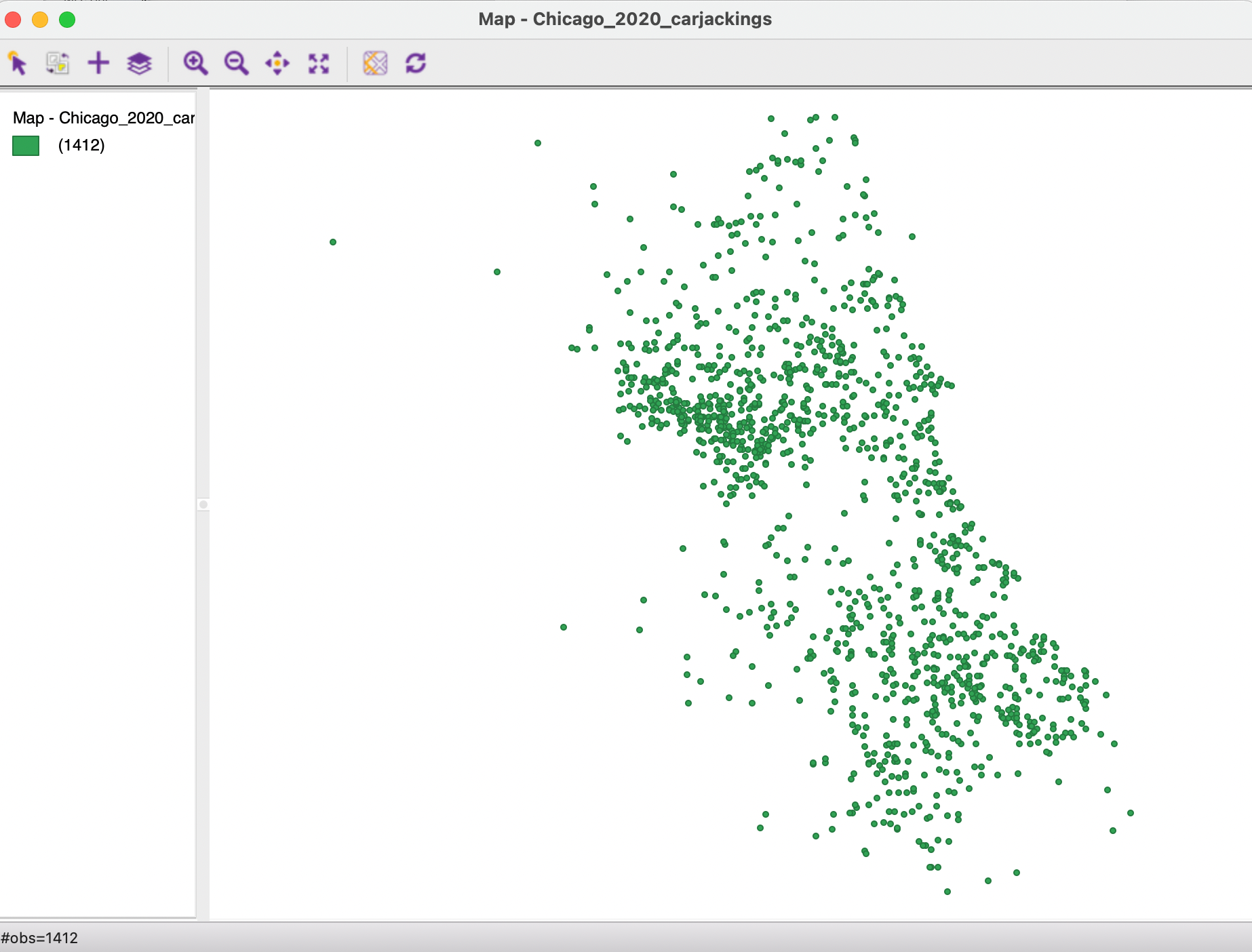
Figure 2.11: Point layer from coordinates

The outline of Chicago suggested by the points is different from the one in Figure 2.7. Again, this is due to the difference in projections, which is discussed next.

At this stage, the point layer can be saved as a GIS file, such as a shape file, using the familiar File > Save As command (the file name should differ from any existing carjackings point shape file, or the latter will be overwritten).

2.3.1.1 A first note about projections

At the bottom of the dialog to save the just created layer is an option to enter CRS (proj4 format). This refers to the projection information, or, more precisely, to the coordinate reference system. Projections will be covered in more detail in the next chapter, but at this point it is useful to be aware of the implications.

As mentioned, a careful comparison of the point pattern in Figure 2.11 and in Figure 2.7 reveals that they are not identical. While the relative positions of the points are the same, they appear more spread out in Figure 2.11. The reason for the discrepancy is the use of different projections. The point shape file in Figure 2.7 is based on the projected X-Y coordinates, whereas the just created point layer uses the latitude-longitude decimal degrees.

As a default, the Coordinate Reference System (CRS) entry in the file save dialog will be empty, as in Figure 2.12. In other words, since nothing was specified other than the coordinates, there is no projection information. As a result, if the layer was saved as a shape file, it would not include a file with a prj file extension.

Figure 2.12: Blank CRS

The lack of projection information severely hampers a range of data manipulations. Specifically, for computations such as Euclidean (straight line) distance, the decimal degrees are inappropriate and either special calculations must be used (such as great circle distance), or the coordinates need to be reprojected.

Even though latitude-longitude decimal degrees are not an actual projection, there is a corresponding CRS. While in and of itself this information is not that meaningful, including it when saving the file makes future reprojections easy. The CRS in proj4 format for decimal degrees is (this is discussed in more detail in the next chapter):

+proj=longlat +datum=WGS84 + no_defs.

Including this entry in the CRS box (see Figure 2.13) when saving the file will ensure that future reprojections will be possible.

Figure 2.13: CRS with projection information

In other words, in the absence of specific projection information, the best practice is to create a spatial layer using decimal latitude-longitude degrees and recording the CRS from Figure 2.13 when saving the information as a GIS format file.

This is pursued in greater technical detail in the next chapter.

2.3.2 Grid

The second type of spatial layer that can be created is a set of grid cells. Such cells are rarely of interest in and of themselves, but are useful to aggregate counts of point locations in order to calculate point pattern statistics, such as quadrat counts.

The grid creation is one of the few instances where GeoDa functionality can be invoked from the menu or toolbar without any table or layer open. From the menu, Tools > Shape > Create Grid brings up a dialog that contains a range of options, shown in Figure 2.14. The most important aspect to enter is the Number of Rows and the Number of Columns, listed under Grid Size at the bottom of the dialog. This determines the number of observations. In the example, the entries are 10 rows and 5 columns, for 50 observations.

There are four options to determine the Grid Bounding Box, i.e., the rectangular extent of the grids. The easiest approach is to use the bounding box of a currently open layer or of an available shape data source. The Lower-left and Upper-right corners of the bounding box can also be set manually, or read from an ASCII file.

In the example in Figure 2.14, the Chicago community area boundary layer, contained in the Chicago_community_areas.shp file is shown as the source for the bounding box.

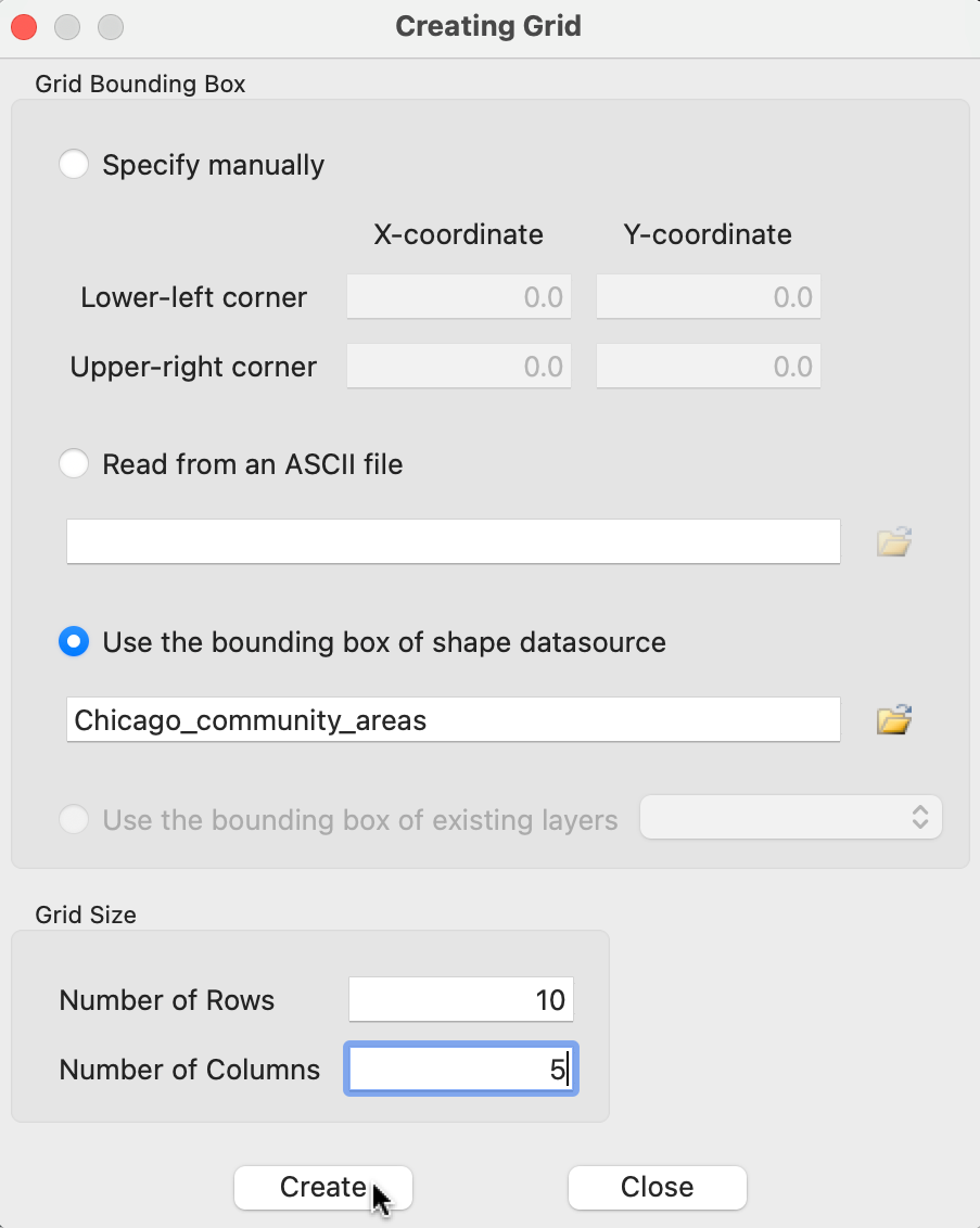
Figure 2.14: Grid creation dialog

After the grid layer is saved as a file, it can be loaded into GeoDa. In Figure 2.15, the result is shown, superimposed onto the community areas layer (how to implement this will be covered in the next chapter). Clearly, the extent of the grid cells matches the bounding box for the area layer.

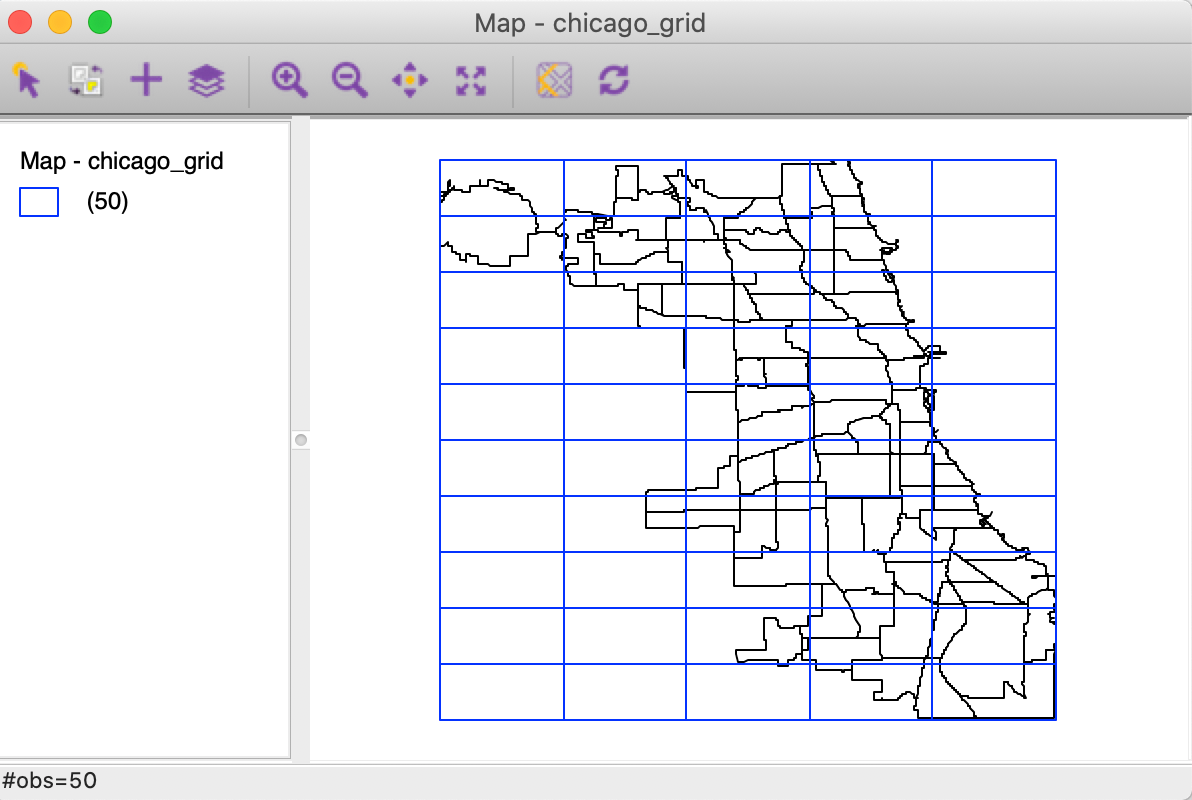
Figure 2.15: Grid layer over Chicago community areas