12.2 Spatial Weights as Distance Functions
In the creation of distance band or k-nearest neighbor weights, the pairwise distance between neighbors is included in the GWT file (see Figure 11.5). However, these values are not used in any actual operations.
The distances themselves are not that useful, but transformations of distance lead to weights that enable spatial transformations. Two types of such functions are considered here: inverse distance weights and kernel weights.
12.2.1 Inverse Distance Weights
Spatial weights based on a distance cut-off can be viewed as representing a step function, with a value of 1 for neighbors with \(d_{ij} < \delta\), and a value of 0 for others. As before, \(d_{ij}\) stands for the distance between observations \(i\) and \(j\), and \(\delta\) is the bandwidth.
A straightforward extension of this principle is to specify the spatial weights as a continuous parameterized function of distance itself: \[\begin{equation} w_{ij} = f(d_{ij},\mathbf{\theta}), \end{equation}\] with \(f\) as a functional form and \(\mathbf{\theta}\) a vector of parameters.
In order to conform to Tobler’s first law of geography, a distance decay effect must be respected. In other words, the value of the function of distance needs to decrease with a growing distance. More formally, this is expressed by the requirement that the partial derivative of the distance function with respect to distance should be negative: \[\partial w_{ij} / \partial d_{ij} < 0.\]
Commonly used distance functions are the inverse, with \(w_{ij} = 1 / d_{ij}^{\alpha}\) (and \(\alpha\) as a parameter), and the negative exponential, with \(w_{ij} = e^{-\beta d_{ij}}\) (and \(\beta\) as a parameter). The functions are typically combined with a distance cut-off criterion, such that for \(d_{ij} > \delta\), it follows that \(w_{ij} = 0\).
In practice, the parameters are often not estimated, but instead set to a fixed value, such as \(\alpha = 1\) for inverse distance weights (\(1/d_{ij}\)), and \(\alpha = 2\) for gravity weights (\(1/d_{ij}^{2}\)). By convention, the diagonal elements of the spatial weights are set to zero and not computed. In fact, if the actual value of \(d_{ii} = 0\) were used in the inverse distance function, this would result in a division by zero.
An often overlooked feature in the computation of distance functions is that the resulting values depend not only on the parameter value and functional form, but also on the metric and scale used for the distance measure. Since the weights are inversely related to distance, large values for the latter will yield small values for the former, and vice versa. This may be a problem in practice when the distances are so large (i.e., measured in small units) that the corresponding inverse distance weights become close to zero, possibly resulting in an all zero spatial weights matrix. This issue is directly related to the scale of the coordinates. It is a common concern in practice when a projection yields distances expressed in feet or meters.
In addition, a potential problem may occur when the distance metric is such that distances take on values less than one. As a consequence, some inverse distance values may be larger than one, which is typically not a desired result.
A simple rescaling of the coordinates on which the distance computation is based will fix both problems.
12.2.1.1 Implementation
Inverse distance weights are specified through the Weights File Creation interface, with the Distance Weight tab selected, as in Figure 11.3. The check box next to Use inverse distance? enables this functionality. This also activates the Power drop down list, where a coefficient can be specified, the default being 1.
The remainder of the interface works in the same fashion as before, with a query for a file name for the new weights.
Using the Italy Community Banks sample data with the default settings yields a spatial weights file like italy_banks_te_id1, the summary properties of which are shown in Figure 12.1. The descriptive statistics are identical to those for the distance band weights in Figure 11.4. The only differences are that inverse distance takes on the value of true, and the power is listed as 1.
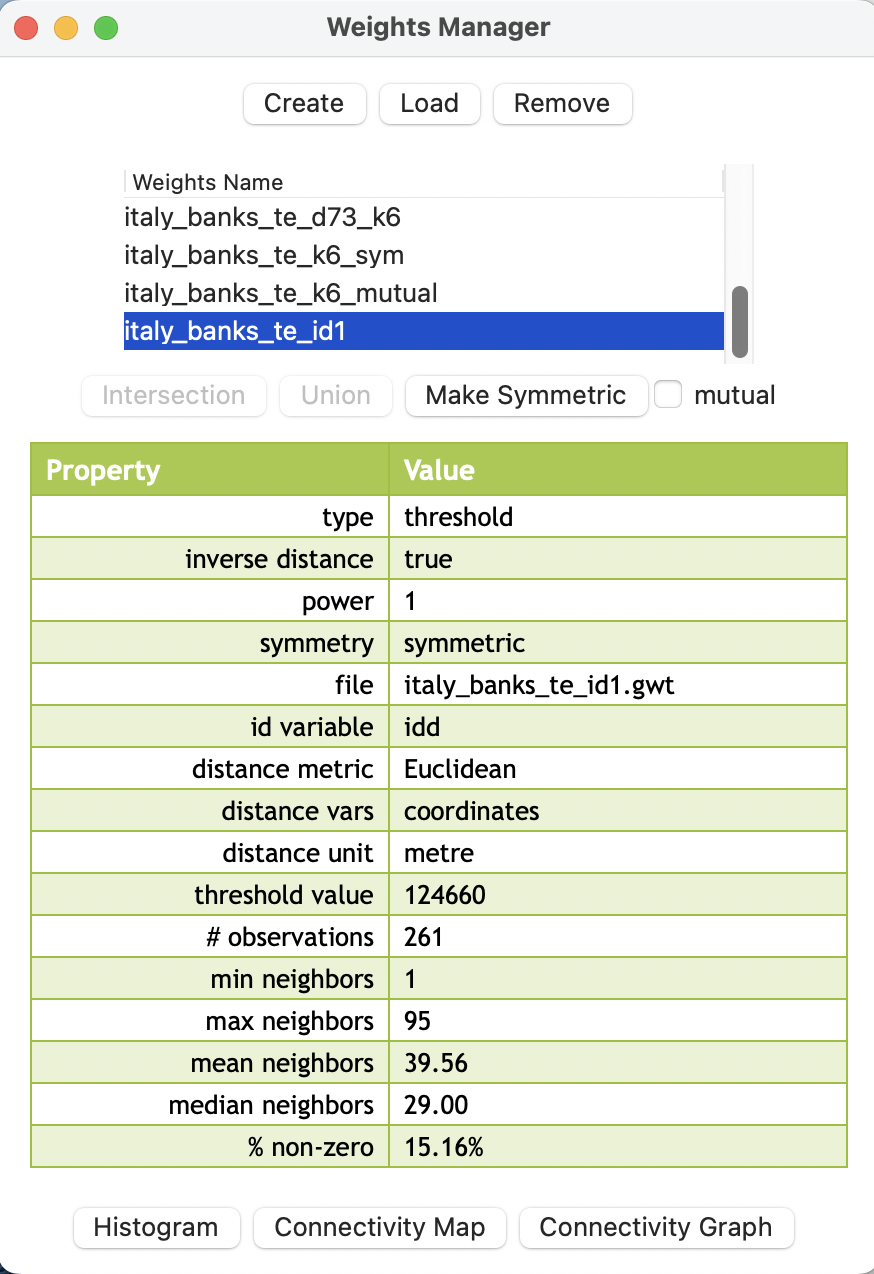
Figure 12.1: Summary properties of inverse distance weights
By design, GeoDa only takes into account the existence of a neighbor relation. The actual values of the weights are ignored. Consequently, the properties of any distance function (irrespective of the power) will be identical to those of the corresponding simple weights
for the same distance band. Also, the connectivity histogram, connectivity map and connectivity graph will be the same as before. They do not provide any new information.
Inverse distance weights can be calculated for any bandwidth specified. While the default is the max-min bandwidth, in some applications this is not useful. For example, the bandwidth can be set to the maximum inter-point distance. As a result, the calculations will be for a full \(n \times n\) distance matrix. This is not recommended for larger data sets, but it can provide a useful point of departure to compute accessibility indices formulated as spatially lagged variables (see Section 12.3.1).
In addition, the coordinate option is perfectly general, and any two variables contained in the data set can be specified as X and Y coordinates in the distance band setup. For example, this allows for the computation of so-called socio-economic weights, where the inverse operation is applied to the Euclidean distance computed in the attribute domain between two locations, using any two (but only two) variables.
In contrast, with the Variables tab checked in the Weights File Creation interface, fully multivariate inverse distance weights can be computed as well, for as many variables as required. However, for such distances to be meaningful, one has to be mindful of the scale in which the variables are expressed. Standardization is highly recommended.
12.2.1.2 K-nearest neighbor inverse distance weights
The computation of inverse distance weights extends to the k-nearest neighbor design in a straightforward manner. The only difference is that the K-Nearest neighbors tab must be checked. All the operations are the same as for distance band weights.
For example, using the original coordinates with k=6, this yields a GWT file, e.g., italy_banks_te_idk6.gwt, and with the coordinates in kilometers, a file italy_banks_te_idk6km.gwt.
12.2.1.3 GWT file
The results of an inverse distance calculation are written to a GWT file, which has the same structure as before. However, in contrast to the standard case, the third column now contains the value for the inverse distance rather than the distance itself.
To illustrate this, consider the two GWT files just created, using 6 nearest neighbors as the bandwidth. The left-hand panel of Figure 12.2 shows the outcome when using the default coordinates (italy_banks_te_idk6.gwt). Note how the value of 2.01549423e-05 for the pair 1-95 is exactly the inverse of the distance of 49,615.6221 (meters), listed on the matching line of Figure 11.5.
This illustrates the problem just mentioned. Since the projected coordinates for the Italian bank point file are expressed in meters, the distances are fairly large (e.g., almost 50 km in the example). As a consequence, the values obtained for inverse distance are very small. This has undesirable effects for the computation of spatial transformations like a spatially lagged variable.
The right-hand panel in Figure 12.2 shows the result after the coordinates were rescaled to kilometers.87 The outcome is simply multiplied by 1,000.
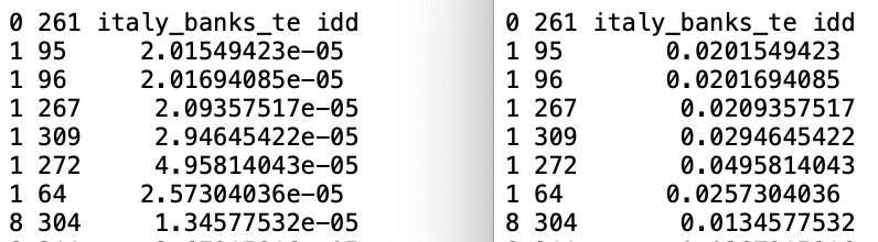
Figure 12.2: GWT files with distance for original and rescaled coordinates
12.2.2 Kernel Weights
Kernel smoothing is a core element in nonparametric statistics (Silverman 1986; Racine 2019). It is essentially a weighted average of observations, centered on a focal point, with decreasing weights as the distance to the focal point increases. The magnitude of the weights is determined by a kernel function, i.e., a decreasing function of the distance to the focal point (in attribute space), and a bandwidth, i.e., the range within which observations are weighted.
In spatial analysis, kernel weights are probably best known for their inclusion in geographically weighted regression, or GWR (Fotheringham, Brunsdon, and Charlton 2002). However, they are also an essential part of non-parametric approaches to model spatial covariance (Hall and Patil 1994), considered more closely in Chapter 13.88
More precisely, kernel weights are defined as a function \(K(z)\) of the ratio between the distance \(d_{ij}\) from \(i\) to \(j\), and the bandwidth \(h_i\), with \(z = d_{ij} / h_i\). This ensures that \(z\) is always less than 1. For distances greater than the bandwidth, \(K(z) = 0\).
Two important considerations in the use of kernel weights are the selection of the kernel function and the determination of the bandwidth.
12.2.2.1 Specification of the kernel weights
Kernel functions determine how quickly the weights get smaller as the distance to the focal point increases. In GeoDa, there currently is support for five
commonly used kernel weights functions:
- Uniform, \(K(z) = 1/2\) for \(|z| < 1\),
- Triangular, \(K(z) = (1 - |z| )\) for \(|z| < 1\),
- Quadratic or Epanechnikov, \(K(z) = (3/4) (1 - z^2)\) for \(|z| < 1\),89
- Quartic, \(K(z) = (15/16)(1 - z^2)^2\) for \(|z| < 1\), and
- Gaussian. \(K(z) = (2 \pi)^{(-1/2)} \exp(- z^2 / 2)\).90
Typically, the value for the diagonal elements of the weights is set to 1, although sometimes the actual kernel value is used. For example, for a quadratic of Epanechnikov kernel function, the weight for \(d_{ij} = 0\) would in principle be \(3/4\), although in practice a value of \(1\) is often used as well.
Many careful decisions must be made in selecting a kernel function. Apart from the choice of a functional form for \(K(\ )\), a crucial aspect is the selection of the bandwidth. In the literature, the latter is found to be more important than the functional form. Several rules have been developed to determine an optimal bandwidth (e.g., see Silverman 1986), although in practice, trial and error may be more appropriate.
An important choice is whether the bandwidth should be the same for all observations, a so-called fixed bandwidth, or instead allowed by vary, as a variable bandwidth.
A drawback of fixed bandwidth kernel weights is that the number of non-zero weights can differ considerably from one observation to the next, especially when the density of the point locations is not uniform throughout space. This is the same problem encountered for the distance band spatial weights (Section 11.3.1).
GeoDa includes two different implementations of the concept of fixed bandwidths. One is the max-min distance used earlier (the largest
of the nearest-neighbor distances). The other is the maximum distance
for a given specification of k-nearest neighbors. For example, for a specified number
of nearest neighbors, this is the distance between the k-nearest
neighbors pairs that are the farthest apart. In other words, this is an extension of the max-min concept to the specific context of k neighbors, rather than nearest neighbor pairs.
To correct for the issues associated with a fixed bandwidth, a variable bandwidth approach can be taken. It adjusts the bandwidth for each location to ensure equal or near-equal coverage. One common approach is to take the k-nearest neighbors, and to adjust the bandwidth for each location such that exactly k neighbors are included in the kernel function. The bandwidth specific to each location is then any distance larger than its k nearest neighbor distance, but less than the k+1 nearest neighbor distance.
When the kernel weights are implemented for the nearest neighbor concept, a final
decision pertains to the value of k. In GeoDa, the default value for k equals the cube root of the number
of observations.91. In general,
a wider bandwidth gives smoother and more robust results, so the bandwidth
should always be set at least as large as the recommended default. Some experimentation may be needed to find a suitable combination of bandwidth and/or number of nearest neighbors in each particular application.
12.2.2.2 Creating kernel weights
Kernel weights are created with the Distance Weight tab in the Weights File Creation interface. The Method must be specified as Kernel, as shown in Figure 12.3. In this illustration for the Italian community bank example, the coordinates have been converted to kilometers, specified as XKM and YKM.
The Kernel functionality brings up several options, as illustrated in the figure. The Kernel function drop down list contains the five supported functions. In the example, the Epanechnikov kernel is selected. Furthermore, the actual weights are used for the diagonal elements, with the radio button checked next to Apply kernel to diagonal weights. The default is actually to have Diagonal weights = 1.
The next set of options pertains to the bandwidth. The default max-min distance is listed in the Specify bandwidth box as 124.659981 km. In the example, the Adaptive bandwidth is checked, with 7 neighbors. A final option is to instead specify a fixed bandwidth with max knn distance as bandwidth.

Figure 12.3: Kernel weights in Weights File Creation interface
The suggested value of k in the interface is based on the cube root criterion. In the example, this is the cube root of 261, or 6.39, rounded up to the next integer (7). Note that the convention used in GeoDa is to count the observation itself as one of k, so that in fact only k-1 true nearest neighbors are taken into account.
The result is saved in a file with a KWT extension, e.g., italy_banks_te_epa.kwt, for consistency with the approach taken in the PySAL library. Except for the inclusion of the diagonal element, its structure is the same as a GWT format file.
12.2.2.3 Characteristics of kernel weights
As soon as the weights are created, their properties appear in the weights manager. As illustrated in Figure 12.4, the descriptive statistics are again the same as for standard knn weights. The differences are in the first six items. The type of weights is given as kernel, the kernel method is identified as Epanechnikov, with the bandwidth definition (knn 7) and adaptive kernel set to true. It is also indicated that the kernel is applied to the diagonal elements, since kernel to diagonal is true. Also, as for the k-nearest neighbor weights, the resulting weights are asymmetric.
Since the connectivity histogram, map and graph ignore the actual weights values and are solely based on the implied connectivity structure, they are identical to those obtained for the corresponding k-nearest neighbor weights. Consequently, they are not informative with respect to the properties of the weights themselves.
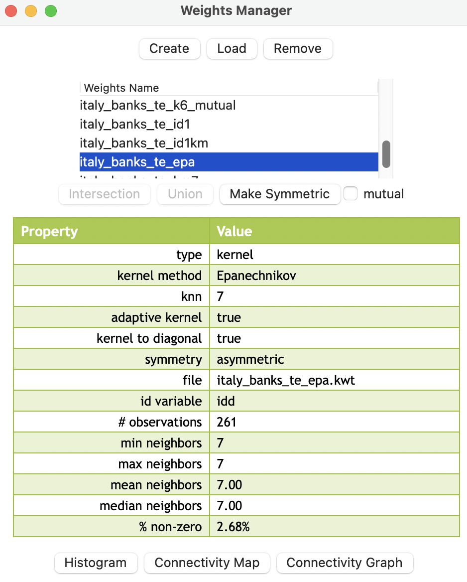
Figure 12.4: Properties of kernel weights
12.2.2.4 KWT file
The contents of the KWT file in our example are shown in the right-hand panel of Figure 12.5, compared to the knn distances in the corresponding GWT file on the left (based on coordinates expressed as kilometers).
A few characteristics of the results should be noted. First, the bandwidth is determined by the largest distance among the seven neighbors. In the current example, for observation 1, the panel on the left shows the distance to the seventh neighbor (249) as 54.251 km. This is the bandwidth. As a result, the kernel weight value for the link 1 to 249 will be 0 (right hand panel). The value for \(z\), to be used in the kernel function, is therefor obtained by dividing the pairwise distances by 54.251. For example, for the link between 1 and 95, who are 49.615 km apart, this yields 0.915. The value for the Epanechnikov kernel is \(0.75(1 - z^2) = 0.75 (1 - 0.836) = 075 \times 0.164 = 0.123\), the result listed in the third column of the matching row on the right-hand side.
There are eight entries for observation 1: the seven neighbors as well as the diagonal. For the latter, listed as the pair 1 to 1, the value is 0.75.
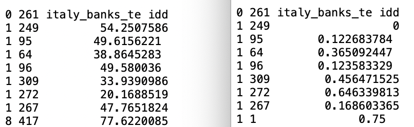
Figure 12.5: KWT file
In
GeoDa, this is implemented in the Calculator. Assuming that COORD_X and COORD_Y are the coordinates in meters, a new set of variables XKM and YKM are computed by dividing these values by 1,000. The new XKM and YKM then need to be entered as respectively X_coordinate variable and Y_coordinate variable in the Weights File Creation interface.↩︎An application in spatial econometrics is the heteroskedasticity and autocorrelation consistent (HAC) estimation of the regression error variance, due to Kelejian and Prucha (2007). See Anselin and Rey (2014), for implementation details in GeoDaSpace and PySal.↩︎
Note that the Epanechnikov kernel is sometimes referred to without the (3/4) scaling factor.
GeoDaimplements the scaling factor.↩︎While the Gaussian kernel is in principle without a bandwidth constraint, in
GeoDait is implemented with the same bandwidth option as the other kernel functions.↩︎This is based on the recommendation by Kelejian and Prucha (2007) in the context of HAC estimation and typically forms a good starting point↩︎