3.3 Converting Between Points and Polygons
So far, the geography of the community areas has been represented by their actual boundaries. However, this is not the only possibility. Equivalently, a representative point for each area can be specified, such as a mean center or a centroid. In addition, new polygons can be constructed to represent the community areas as tessellations around those central points, such as Thiessen polygons. The key factor is that all three representations are connected to the same cross-sectional data set. As discussed in more detail in later chapters, for some types of analyses it is advantageous to treat the areal units as points, whereas in other situations Thiessen polygons form a useful alternative to dealing with an actual point layer.
The center point and Thiessen polygon functionality is invoked through the options menu associated with the map view (right click on the map to bring up the menu). This is illustrated with the just created projected community area map (Figure 3.4).
3.3.1 Mean centers and centroids
Two concepts are in common use to represent the center of a polygon. One is the mean center, which is simply the (unweighted) average of the coordinates of the vertices, so \((1/k) \sum_i x_i\) and \((1/k) \sum_i y_i\) (where \(k\) is the number of vertices). The notion of a centroid is more complex, as it represents the center of gravity of the polygon. A classic exercise is to create a cutout of the polygon and to find the centroid as the location where a pin would hold it up in a stable equilibrium.
The main difference between the mean center and the centroid is that the latter takes into account the area of the polygon. It is computed as an area weighted average of the centers of the set of triangles that represent the polygon. This so-called triangulation of a polygon is a standard operation in computational geometry (see, for example, Worboys and Duckham 2004; de Berg et al. 2008). Once the triangulation is obtained, the centers of the triangles (the average of their coordinates) and their areas can be readily computed to obtain the centroid.16
The calculation of the mean center and centroid can yield strange results when the polygons are highly irregular (not convex), have holes, or represent a so-called multi-polygon situation (different polygons associated with the same ID, such as a mainland area and an island belonging to the same county). In those instances, the centers can end up being located outside the polygon. Nevertheless, the shape centers are a handy way to convert a polygon layer to a corresponding point layer with the same underlying geography. For example, as covered in Chapter 11, they are used under the hood to calculate distance-based spatial weights for polygons.
3.3.1.1 Shape Center options
In GeoDa, the Shape Center option from the map view has three main functions, applied to either the Mean Centers or the Centroids. These are: Add to Table, Display and Save.
The simplest is to Display the center points on the map. This is purely illustrative and the points are not available for any further manipulation, in contrast with the multi-layer option discussed in Section 3.6. For example, in Figure 3.5, the mean centers of the Chicago community areas are displayed as small circles on top of the default themeless map from Figure 3.4.
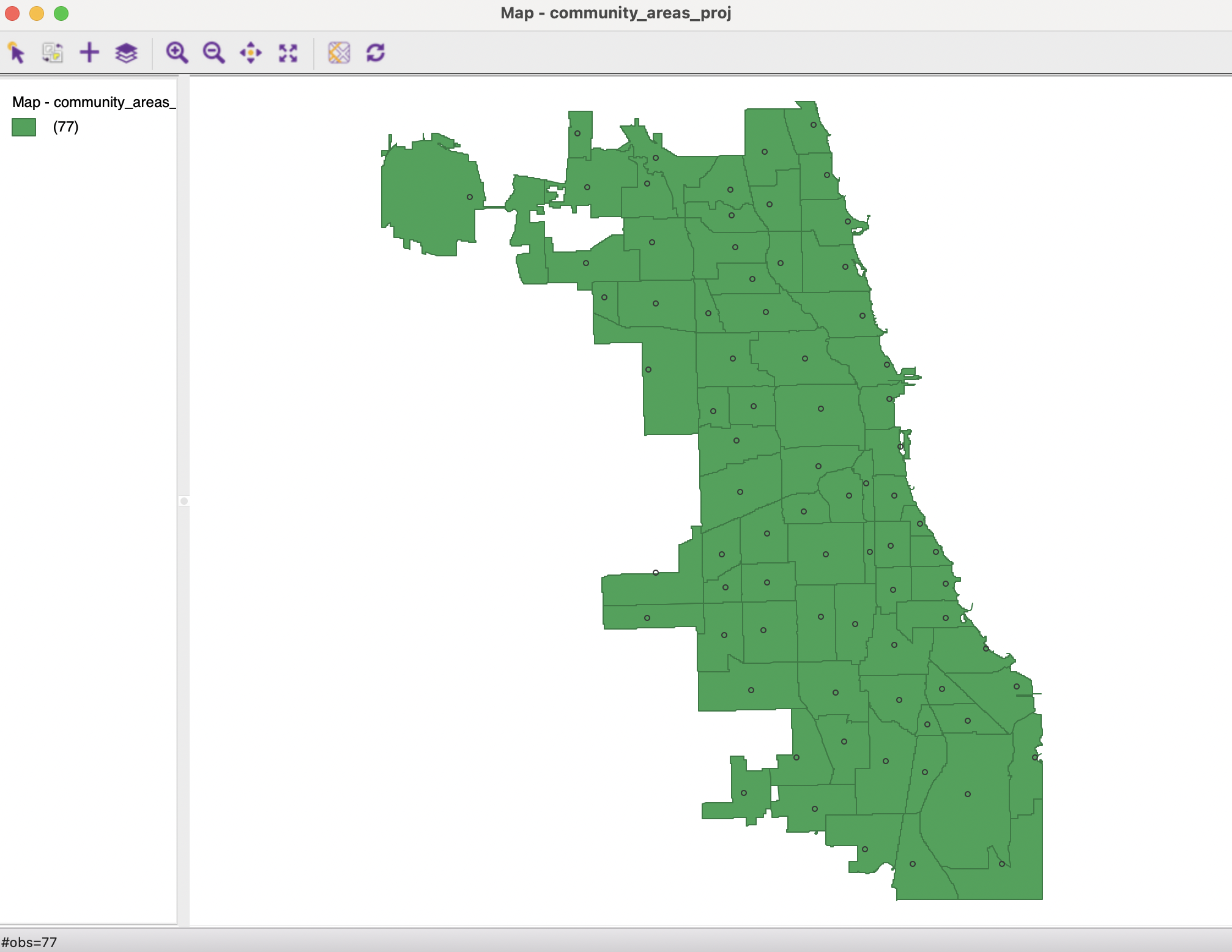
Figure 3.5: Display mean centers on map
A second option is to Add the coordinates of the central points to Table. This brings up a dialog that prompts for the variable names for the coordinates, with COORD_X and COORD_Y as defaults. For example, the mean center coordinates could be set to COORD_XM and COORD_YM and the centroids to COORD_XC and COORD_YC. In Figure 3.6, the associated coordinate values are shown in the table (after some reshuffling of columns). Close examination of the values reveals only minor differences between the two types of mean centers in this particular case, in part because the community areas have mostly fairly convex shapes (the coordinates are in meters).
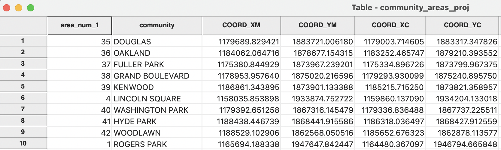
Figure 3.6: Add mean centers to table
Finally, the Save option results in the usual prompt for a file name (e.g., comm_area_centers.shp) and creates the new layer. In the example, the point layer associated with the community area mean centers is as in Figure 3.7.
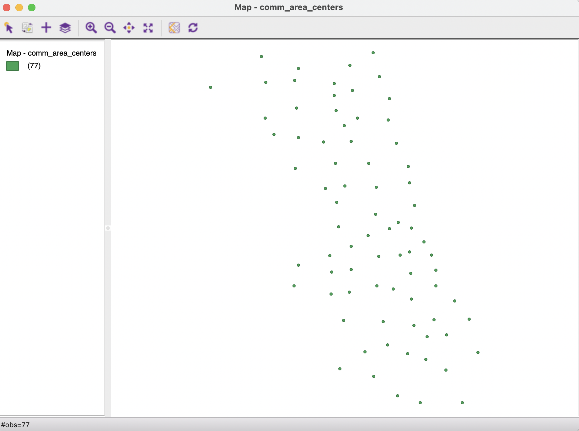
Figure 3.7: Chicago community area mean center layer
3.3.2 Tessellations
A tessellation is the exhaustive covering of an area with polygons or tiles. Of particular interest in spatial analysis are so-called Thiessen polygons or Voronoi diagrams (for an extensive discussion, see Okabe et al. 2000).
Thiessen polygons are a regular tiling of polygons centered around points, such that they define an area that is closer to the central point than to any other point. In other words, the polygon contains all possible locations that are nearest neighbors to the central point, rather than to any other point in the data set.17 The polygons are constructed by considering a line perpendicular at the midpoint to a line connecting the central point to its neighbors. The latter is referred to as Delaunay triangulation and is in fact the dual problem to the tessellation.
In sum, any point layer can be converted to a polygon layer with the same geography by constructing Thiessen polygons around the points.
3.3.2.1 Thiessen Polygons options
The Thiessen Polygons functionality is available as an option in the map view for point layers. As for the mean centers, there are three options, although only two of those are used regularly.
The Display option simply draws the polygons around the points, as shown in Figure 3.8 for the mean center points from Figure 3.7. As in the case of the display of mean centers, the resulting polygons cannot be used for any other operations.
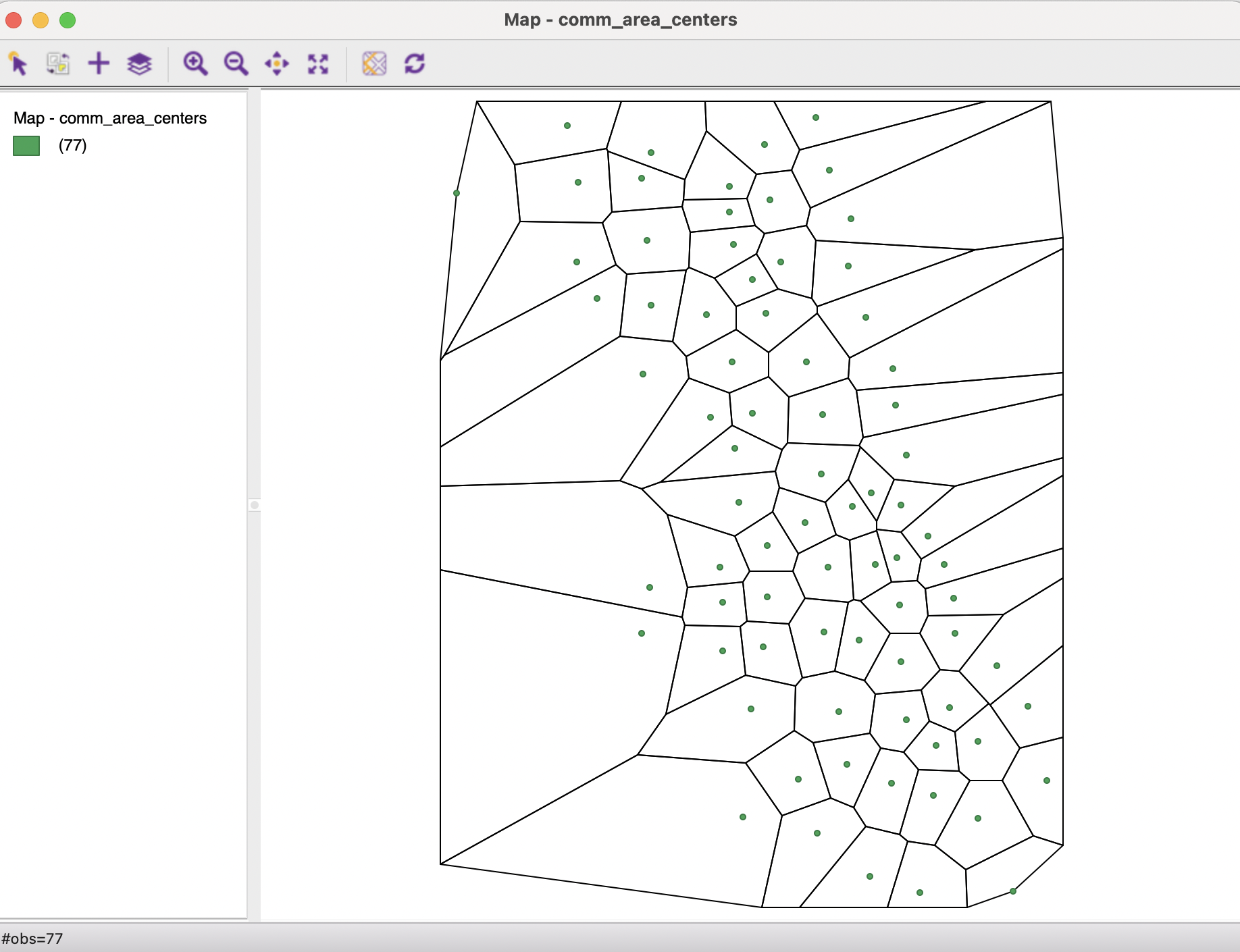
Figure 3.8: Display Thiessen polygons
The Save option will create a new layer with the polygons.18 This layer can then be used in the same way as any other polygon layer, e.g., to create maps or carry out spatial analyses.
GeoDauses the centroid implementation from the GEOS library, see https://libgeos.org/doxygen/classgeos_1_1algorithm_1_1Centroid.html.↩︎In economic geography, this corresponds to the notion of a market area, assuming a uniform distribution of demand.↩︎
A third option is to Save Duplicate Thiessen Polygons to Table. This is only available when there is a problem in the calculation of the polygons due to multiple observations with the same coordinates. This may happen when considering different housing units in a high rise, or when the precision of the coordinates is insufficient to distinguish between all points. The option adds an additional column to the table, labeled DUP_IDS, which contains a value of 1 for those points that have multiple observations with the same coordinates.↩︎