3.4 Minimum Spanning Tree (MST)
3.4.1 Concept
A central concept in the treatment of spatial autocorrelation is the so-called spatial weights matrix, discussed in detail in Part III of this Volume. For now, it is sufficient to know that this matrix shows the neighbor relations between observations. An element of the matrix in row \(i\) and column \(j\), \(w_{ij}\), is non-zero if \(i\) and \(j\) are neighbors (using one of many possible definitions). Technically, this is the same as an adjacency matrix for a graph or network, where the observations are nodes and the non-zero weights correspond to the edges that connect the nodes. In the treatment of spatial weights, the graph structure will be called the connectivity graph.
For example, in Figure 3.9, the connectivity graph is shown for the community area mean centers from Figure 3.7. This graph represents a distance-band weights matrix with a cut-off distance that corresponds to the largest nearest neighbor distance between points, the so-called max-min distance criterion. This ensures that each observation (node) has at least one neighbor.
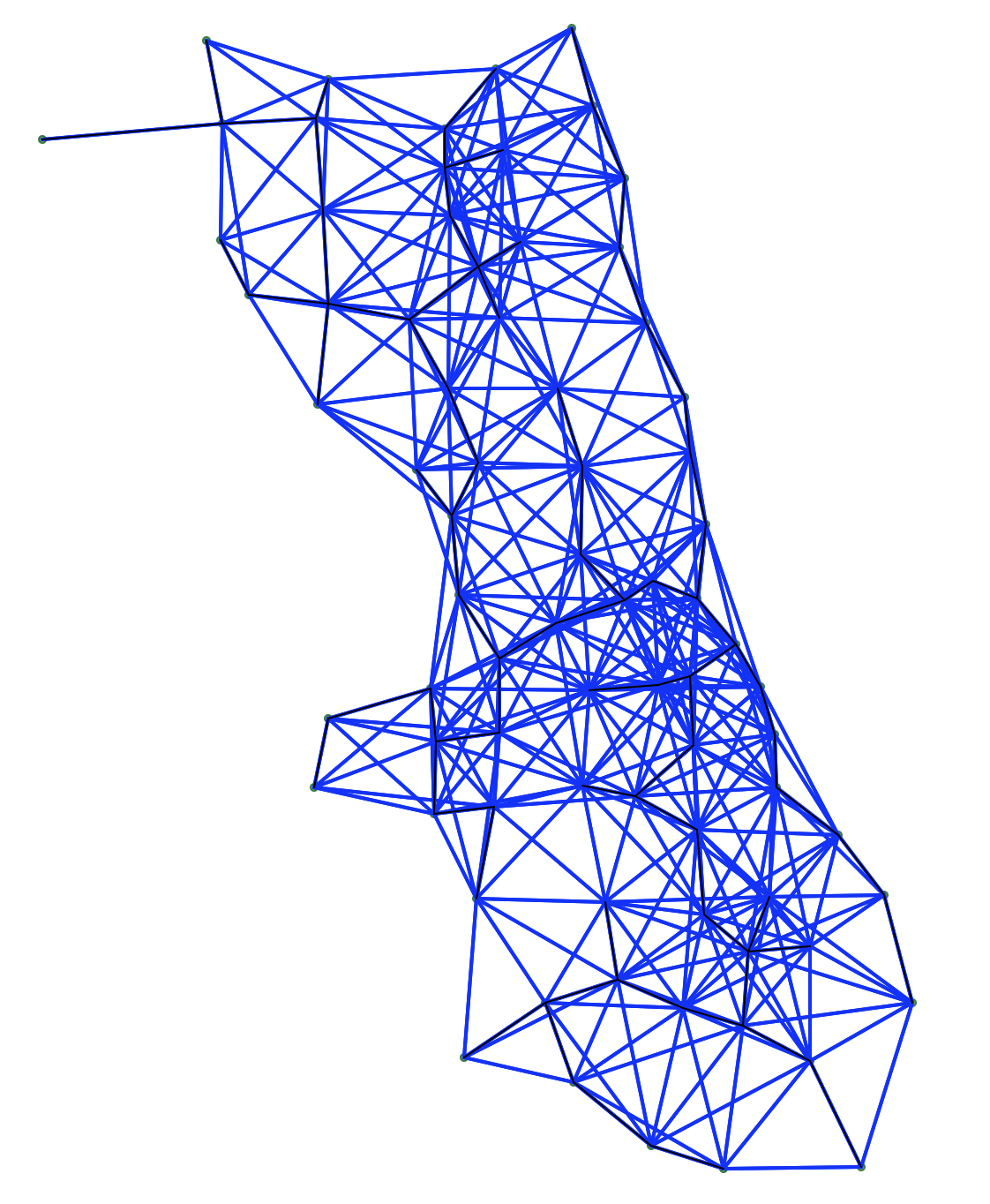
Figure 3.9: Connectivity graph of mean centers
A Minimum Spanning Tree (MST) is a subset of this graph that constitutes a tree, i.e., “a connected, undirected network that contains no loops” (Newman 2018). Importantly, this means that all nodes are connected (no isolates or islands) and there is exactly one path between any pair of nodes (no loops). As a result, a tree associated with \(n\) nodes contains exactly \(n-1\) edges. The MST is a special tree in that the total sum of the edge lengths (typically a weight) is minimized. It constitutes a simplification of the full network structure that fulfills a minimum cost objective.
For example, the MST computed from the network structure in Figure 3.9 is shown in Figure 3.10. The complexity of the graph is greatly reduced and now consists of only 76 edges (for 77 observations or nodes).
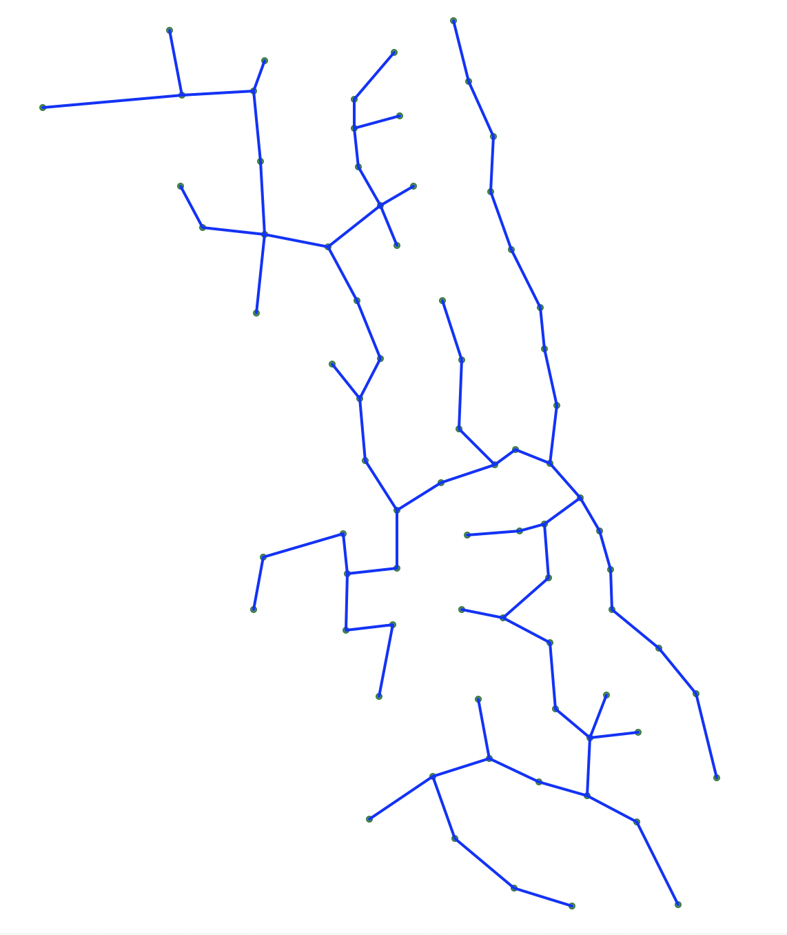
Figure 3.10: Mininum Spanning Tree for Connectivity graph of mean centers
The MST is similar to, but distinct from the solution to the so-called traveling salesperson problem, which looks for a route through the network that achieves a minimum cost objective, but visits each node just once. This implies that the nodes in a solution to the traveling salesperson problem cannot have a degree (i.e., the number of edges connected to it) larger than two. In Figure 3.10, the maximum degree is four.
A classic solution to the MST problem is achieved by Prim’s algorithm (Prim 1957), illustrated in the following worked example. The MST plays a major role in some of the spatial clustering procedures discussed in Volume 2.
3.4.1.1 Worked example - Prim’s algorithm for MST
A small toy example consisting of 9 points is used to illustrate the mechanics of Prim’s MST algorithm. The coordinates of the points are listed in Figure 3.11.
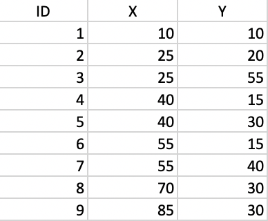
Figure 3.11: Toy example point coordinates
The corresponding inter-point distance matrix is given in Figure 3.12.
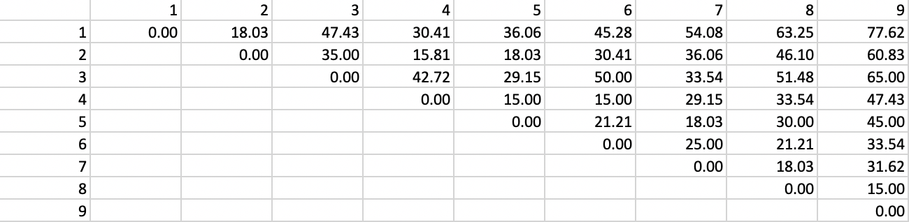
Figure 3.12: Inter-point distance matrix
The inter-point distances form the basis to construct a connectivity graph for a distance band that ensures that each point is connected to at least one other point. In the example, this distance is 29.15.19 The corresponding graph representation is given in Figure 3.13, where each point is a node and the edges show the connections and associated distances.
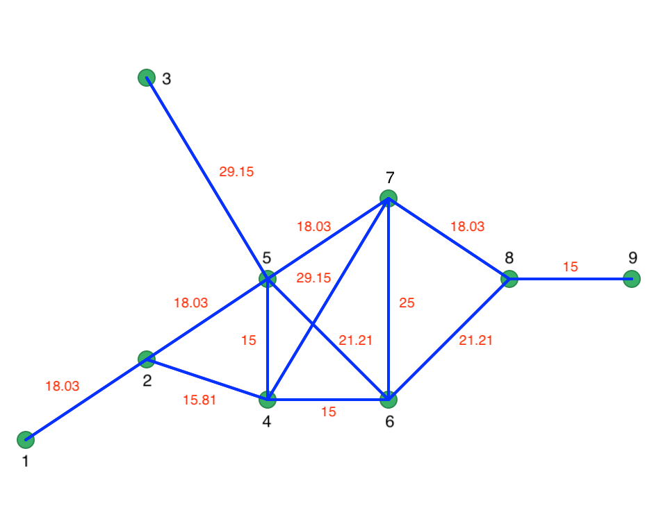
Figure 3.13: Connectivity graph
Prim’s algorithm proceeds by starting at a random node and selecting the shortest edge to the next node. For example, starting with node 1, there is only a single edge, such that the first path is from node 1 to 2. At node 2, there are two edges, 2-4 with length 15.81, and 2-5 with length 18.03. Therefore, the next link is between 2 and 4. At this point, the shortest path follows the red lines as in Figure 3.14.
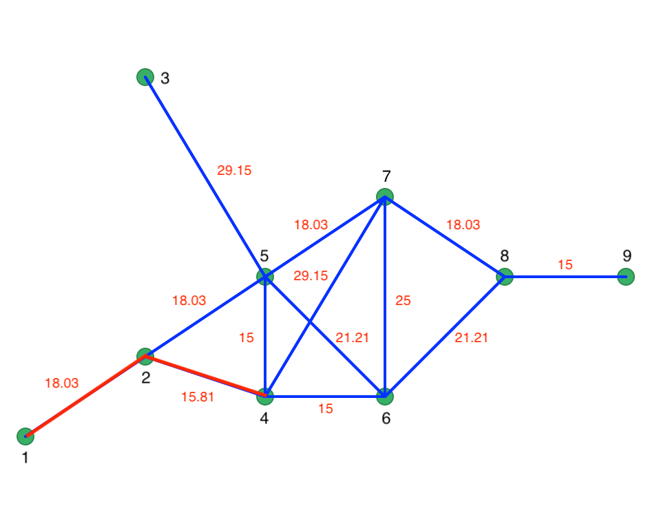
Figure 3.14: Initial steps in Prim’s algorithm
At node 4, the two edges have the same length, so 4 could be connected to either 6 or 5. The order is immaterial, since the length of 15 is the smallest in the network and will have priority over any other edge. At this point, the path consists of 1-2, 2-4, 4-6 and 4-5. The next step connects 5 to 7 (18.03), then 7 to 8 (18.03), and 8 to 9 (15). The only remaining unconnected node is 3, which is linked to 5 (29.15). The resulting MST follows the red lines in Figure 3.15. Every node is visited and the total distance of the path is minimized. The solution consists of eight edges, which is \(n - 1\).
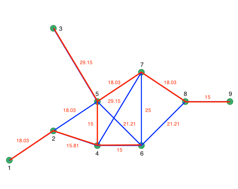
Figure 3.15: Minimum spanning tree
Note that the MST solution is not unique since there can be several trees that achieve the same minimum cost solution.
3.4.2 Minimum Spanning Tree options
Minimum Spanning Tree is one of the entries in the options menu associated with a map view for a point layer (right click on the layer to invoke the menu). There are two main options: Display Minimum Spanning Tree, which simply shows the edges on the point map, and Save Minimum Spanning Tree. The latter saves the MST information in the gwt spatial weights format (see Chapter 11), which makes it available for use in other analyses.
In addition, there are two options to (slightly) change the format of the MST display: Change Edge Thickness (with three options: Light, Normal - the default - and Strong), and Change Edge Color. The display in Figure 3.10 has the Edge Thickness as Strong and the color changed to blue (from the default black).
Connectivity graphs are discussed in more detail in the chapters dealing with spatial weights in Part III.↩︎