6.4 Rate Smoothing
In many empirical investigations, the real interest is in the spatial distribution of the underlying risk of an event. While the concept of risk has many meanings, in this context it represents the probability of an event occurring. To the extent that the risk is not constant across space, its spatial distribution is represented by a so-called risk surface. The problem is that such a surface is not observed and thus must be estimated.
As it turns out, the crude rate is a good estimate for the unknown risk in that it is unbiased (on average, it is on target). However, it suffers from the problem that its precision (or, alternatively, its variance) is not constant and depends on the size of the corresponding population at risk (the denominator). This intrinsic variance instability of rates causes problems for the interpretation of maps, especially in terms of the identification of outliers. In addition, there are challenges to create meaningful maps when dealing with many locations that have no observed events.
In response, a number of procedures have been suggested that trade off some bias in order to increase overall precision, by borrowing strength.
In this section, I first present more formally some important concepts related to variance instability, as well as ways to improve the risk estimates by means of smoothing rates. In the current chapter, the discussion is limited to one particular approach, i.e., Empirical Bayes smoothing. Spatial smoothing methods are covered in Chapter 12.
6.4.1 Variance Instability
The point of departure in the consideration of rate smoothing is to view the count of events that occur in a location \(i\), \(O_i\), as the number of successes in \(P_i\) draws from a probability distribution driven by a risk parameter \(\pi_i\). The textbook analog is to draw \(n\) balls from an urn filled with red and white balls, say with a proportion of \(p\) red balls. Given \(n\) such draws, what is the probability that \(q\) balls will be red?
The formal mathematical framework for this type of situation is the binomial distribution, \(B(n,p)\). The probability function for this distribution gives the probability of \(k\) successes in \(n\) successive draws from a population with risk parameter \(p\): \[\mbox{Prob}[k] = \binom{n}{k} p^k (1 - p)^{n - k},\] where \(\binom{n}{k}\) is the binomial coefficient.40 Translated into the context of \(O_i\) events out of a population of \(P_i\), the corresponding probability is: \[\mbox{Prob}[O_i] = \binom{P_i}{O_i} \pi_i^{O_i} (1 - \pi_i)^{P_i - O_i},\] with \(\pi_i\) as the underlying risk parameter. The mean of this binomial distribution is \(\pi_i P_i\), and the variance is \(\pi_i (1 - \pi_i) P_i\).
Returning to the crude rate \(r_i = O_i / P_i\), it can be readily seen that its mean corresponds to the underlying risk:41 \[E[r_i] = E[\frac{O_i}{P_i}] = \frac{E[O_i]}{P_i} = \frac{\pi_i P_i}{P_i} = \pi_i.\] Consequently, the crude rate is an unbiased estimator for the underlying risk.
However, the variance has some undesirable properties. A little algebra yields the variance as: \[Var[r_i] = \frac{\pi_i (1 - \pi_i) P_i}{P_i^2} = \frac{\pi_i (1 - \pi_i)}{P_i}.\] This result implies that the variance depends on the mean, a non-standard situation and an additional degree of complexity. More importantly, it implies that the larger the population of an area (\(P_i\) in the denominator), the smaller the variance for the estimator, or, in other words, the greater the precision.
The flip side of this result is that for areas with sparse populations (small \(P_i\)), the estimate for the risk will be imprecise (large variance). Moreover, since the population typically varies across the areas under consideration, the precision of each rate will vary as well. This variance instability needs to somehow be reflected in the map, or corrected for, to avoid a spurious representation of the spatial distribution of the underlying risk. This is the main motivation for smoothing rates, considered next.
6.4.2 Borrowing strength
Approaches to smooth rates, also called shrinkage estimators, improve on the precision of the crude rate by borrowing strength from the other observations. This idea goes back to the fundamental contributions of James and Stein (the so-called James-Stein paradox), who showed that in some instances biased estimators may have better precision in a mean squared error sense (James and Stein 1961).
Formally, the mean squared error or MSE is the sum of the variance and the square of the bias. For an unbiased estimator, the latter term is zero, so then MSE and variance are the same. The idea of borrowing strength is to trade off a (small) increase in bias for a (large) reduction in the variance component of the MSE. While the resulting estimator is biased, it is more precise in a MSE sense. In practice, this means that the chance is much smaller to be far away from the true value of the parameter.
The implementation of this idea is based on principles of Bayesian statistics, which are briefly reviewed next.
6.4.2.1 Bayes Law
The formal logic behind the idea of smoothing is situated in a Bayesian framework, in which the distribution of a random variable is updated after observing data.42 The principle behind this is the so-called Bayes Law, which follows from the decomposition of a joint probability (or density) of \(A\) and \(B\) into two conditional probabilities: \[ P[AB] = P[A | B] \times P[B] = P[B | A] \times P[A],\]
where \(A\) and \(B\) are random events, and \(|\) stands for the conditional probability of one event, given a value for the other. The second equality yields the formal expression of Bayes law as: \[P[A | B] = \frac{P[B | A] \times P[A]}{P[B]}.\]
In most instances in practice, the denominator in this expression can be ignored, and the equality sign is replaced by a proportionality sign: \[P[A | B] \propto P[B | A] \times P[A].\]
In the context of estimation and inference, the \(A\) typically stands for a parameter (or a set of parameters) and \(B\) stands for the data. The general strategy is to update what is known about the parameter \(A\) a priori (reflected in the prior distribution \(P[A]\)), after observing the data \(B\), to yield a posterior distribution, \(P[A | B]\), i.e., what is known about the parameter after observing the data. The link between the prior and posterior distribution is established through the likelihood, \(P[B | A]\). Using a more conventional notation with \(\pi\) as the parameter and \(y\) as the observations, this gives:43 \[P[\pi | y] \propto P[y | \pi] \times P[\pi].\] For each particular estimation problem, a distribution must be specified for both the prior and the likelihood. This must be carried out in such a way that a proper posterior distribution results. Of particular interest are so-called conjugate priors, which result in a closed form expression for the combination of likelihood and prior distribution. In the context of rate smoothing, there are a few commonly used priors, such as the Gamma and the Gaussian (normal) distribution.44 A formal mathematical treatment is beyond the current scope, but it is useful to get a sense of the intuition behind smoothing approaches.
In essence, it means that the estimate from the data (i.e., the crude rate) is adjusted with some prior information, such as the reference rate for a larger region (e.g., the state or country). Unreliable small area estimates are then shrunk towards this reference rate. For example, if a small area is observed with zero occurrences of an event, does that mean that the risk is zero as well? Typically, the answer will be no, and the smoothed risk will be computed by borrowing information from the reference rate.
6.4.2.2 The Empirical Bayes approach
The Empirical Bayes approach is based on the so-called Poisson-Gamma model, where the observed count of events (\(O\)) is viewed as the outcome of a Poisson distribution with a random intensity (mean), for example expressed as \(\pi P\). The Bayesian aspect comes in the form of a prior Gamma distribution for the risk parameter \(\pi\). This results in a particular expression for the posterior distribution, which is also Gamma, with mean and variance: \[E[\pi] = \frac{O + \alpha}{P + \beta},\]
and \[Var[\pi] = \frac{O + \alpha}{(P + \beta)^2}\] where \(\alpha\) and \(\beta\) are the the shape and scale parameters of the prior (Gamma) distribution.45
In the Empirical Bayes approach, values for \(\alpha\) and \(\beta\) are estimated from the actual data. The smoothed rate is then expressed as a weighted average of the crude rate, say \(r\), and the prior estimate, say \(\theta\). The latter is estimated as a reference rate, typically the overall statewide average or some other standard.
In essence, the EB technique consists of computing a weighted average between the raw rate for each small area and the reference rate, with weights proportional to the underlying population at risk. Simply put, small areas (i.e., with a small population at risk) will tend to have their rates adjusted considerably, whereas for larger areas the rates will barely change.46
More formally, the EB estimate for the risk in location \(i\) is: \[\pi_i^{EB} = w_i r_i + (1 - w_i) \theta.\]
In this expression, the weights are: \[w_i = \frac{\sigma^2}{(\sigma^2 + \mu/P_i)},\]
with \(P_i\) as the population at risk in area \(i\), and \(\mu\) and \(\sigma^2\) as the mean and variance of the prior distribution. 47
In the empirical Bayes approach, the mean \(\mu\) and variance \(\sigma^2\) of the prior (which determine the scale and shape parameters of the Gamma distribution) are estimated from the data.
For \(\mu\) this estimate is simply the reference rate (the same reference used in the computation of the SMR), \(\sum_{i=1}^{i=n} O_i / \sum_{i=1}^{i=n} P_i\). The estimate of the variance is a bit more complex: \[\sigma^2 = \frac{\sum_{i=1}^{i=n} P_i (r_i - \mu)^2}{\sum_{i=1}^{i=n} P_i} - \frac{\mu}{\sum_{i=1}^{i=n} P_i/n}.\]
While easy to calculate, the estimate for the variance can yield negative values. In such instances, the conventional approach is to set \(\sigma^2\) to zero. As a result, the weight \(w_i\) becomes zero, which in essence equates the smoothed rate estimate to the reference rate.
6.4.3 Empirical Bayes smoothed rate map
In Chapter 5, a unique values map was shown for the cumulative occurrence of Zika in the state of Ceará in 2016. The map in Figure 5.5 indicated that only 32 of the 184 municipios had an incidence of Zika during the period under consideration, meaning that 152 municipalities had no cases. Suggesting that these municipalities therefore had zero risk of exposure to Zika does not seem realistic. Hence the need to borrow some strength from other information.
A crude rate map that uses the cumulative Zika cases (acu_zik_3q) as the Event Variable and the population at risk (pop_zikv) as the Base Variable is shown in the left panel of Figure 6.9 as a quantile map with six categories. Clearly, all but one of the 32 non-zero observations are grouped in the top category, one is the next lower category and everything else is zero.
An Empirical Bayes smoothed map is invoked as Maps > Rates- Calculated Maps > Empirical Bayes in the usual fashion. The same Event Variable and Base Variable are specified and the map type is selected from the same drop down list as in Figure 6.3. The resulting six category quantile map is shown in the right panel of Figure 6.9. The contrast with the crude rate map is striking. Each category has the required 31 or 32 observations, and the map shows much more spatial variety than before. Areas that had zero observations are shrunk towards an average rate, either below or above the median. The highlighted municipalities in the map (blue rectangle) shown three small areas whose smoothed rates pulled the original zero value above the median.
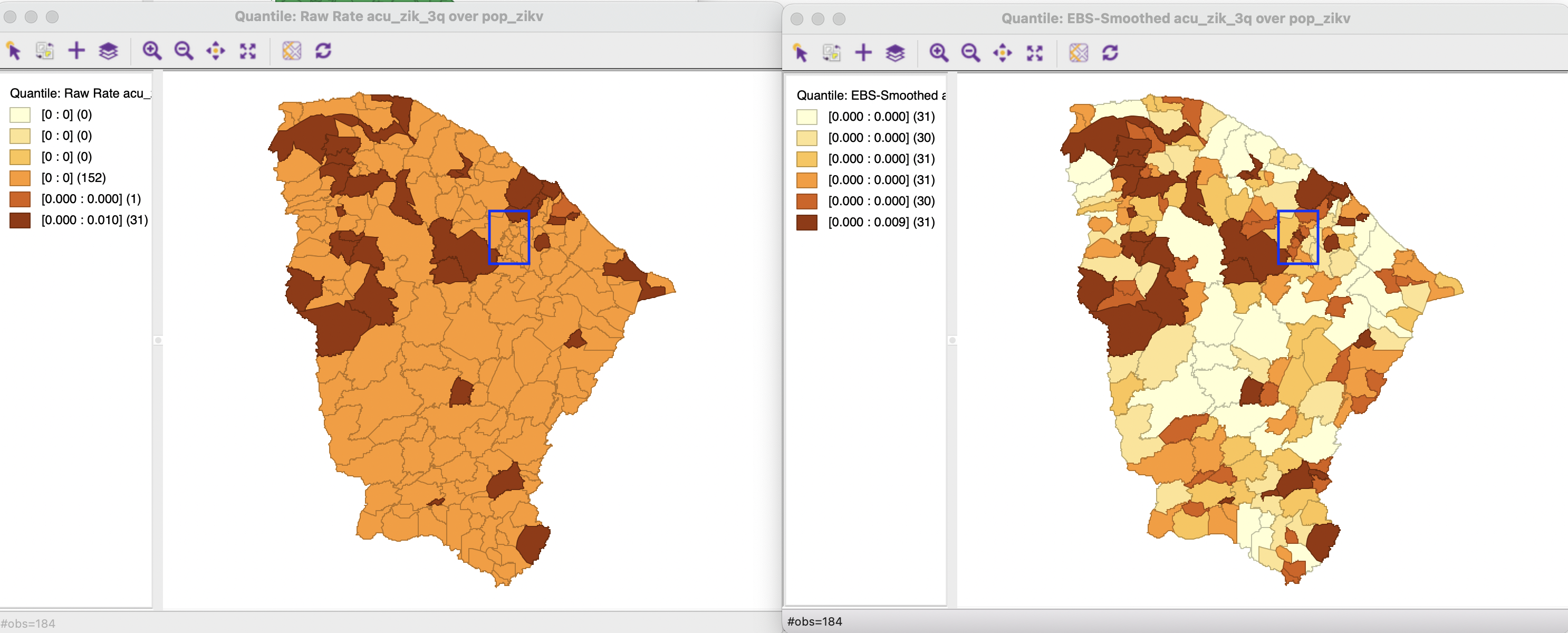
Figure 6.9: Crude and EB rate map
6.4.3.1 The effect of smoothing
In the Ceará example, the total cumulative number of Zika cases was 2,262, for a total population of 8,904,459. This yields a reference rate of 0.000254, or 25.4 per 100,000. The effect of Empirical Bayes smoothing is that the original crude rate is moved towards this overall rate as a function of its population: areas with large populations do not see much change, whereas areas with small populations can take on very different smoothed value.
In Figure 6.10, the effect on small areas is illustrated. The municipalities are ordered by population size, with the 10 smallest areas listed. This clearly illustrates how the crude rate (R_RAW_RT) gets moved towards the overall mean in the Empirical Bayes rate (R_EBS). For example, for the smallest area, the crude rate of zero becomes 5.5 per 100,000 and most of the other crude rates get pulled up towards the overall mean. For the municipio of Altaneira, the opposite happens, i.e., the crude rate of 27.2 per 100,000 becomes 27.0 per 100,000, pulling it down towards the overall mean.
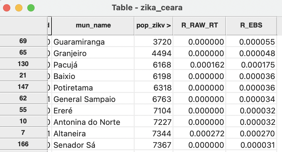
Figure 6.10: Effect of smoothing - small populations
For areas with large populations, there is a minimal effect of the smoothing. Figure 6.11 lists the ten largest municipalities with their crude and smoothed rates. The difference between the two is marginal.
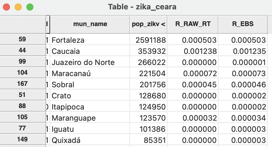
Figure 6.11: Effect of smoothing - large populations
6.4.3.2 Calculating EB smoothed rates in the table
Just as for the other rate maps, the calculated Empirical Bayes smoothed rate can be saved to the table (the default variable name is R_EBS). In addition, the smoothed rates can be computed directly by means of the Calculator option in the Table, following the same procedures as outlined in Section 6.2.2.1.
\(\binom{n}{k} = n! / k!(n-k)!\), or the number of different combinations of \(k\) observations out of \(n\).↩︎
Only the number of observed events \(O_i\) is random, the population size \(P_i\) is not.↩︎
There are several excellent books and articles on Bayesian statistics, with Gelman et al. (2014) as a classic reference.↩︎
Note that in a Bayesian approach, the likelihood is expressed as a probability of the data conditional upon a value (or distribution) of the parameters. In classical statistics, it is the other way around.↩︎
For an extensive discussion, see, for example, the classic papers by Clayton and Kaldor (1987) and Marshall (1991).↩︎
A Gamma(\(\alpha, \beta\)) distribution with shape and scale parameters \(\alpha\) and \(\beta\) has mean \(E[\pi] = \alpha / \beta\) and variance \(Var[\pi] = \alpha / \beta^2\).↩︎
For an extensive technical discussion, see also Anselin, Lozano-Gracia, and Koschinky (2006).↩︎
In the Poisson-Gamma model, this turns out to be the same as \(w_i = P_i / (P_i + \beta)\).↩︎