2.5 Queries
While queries of the data are somewhat distinct from data wrangling per se, drilling down the data is often an important part of selecting the right subset of variables and observations. In order to select particular observations or rows in the data table, the Selection Tool is used. This is arguably one of the most important features of the table options.
The Chicago Carjackings data set is used to illustrate the selection functionality. First, a few adjustments are needed: the Date column must be reformatted to datetime, and new variables for the Month and the Day must be included (using Table > Calculator as in Section 2.4.2.5).
2.5.1 Selection Tool
Queries can be carried out by invoking Table > Selection Tool or right clicking on the table to select this option. The interface, shown in Figure 2.24, supports quite complex searches and operations, even though it may seem somewhat rudimentary.
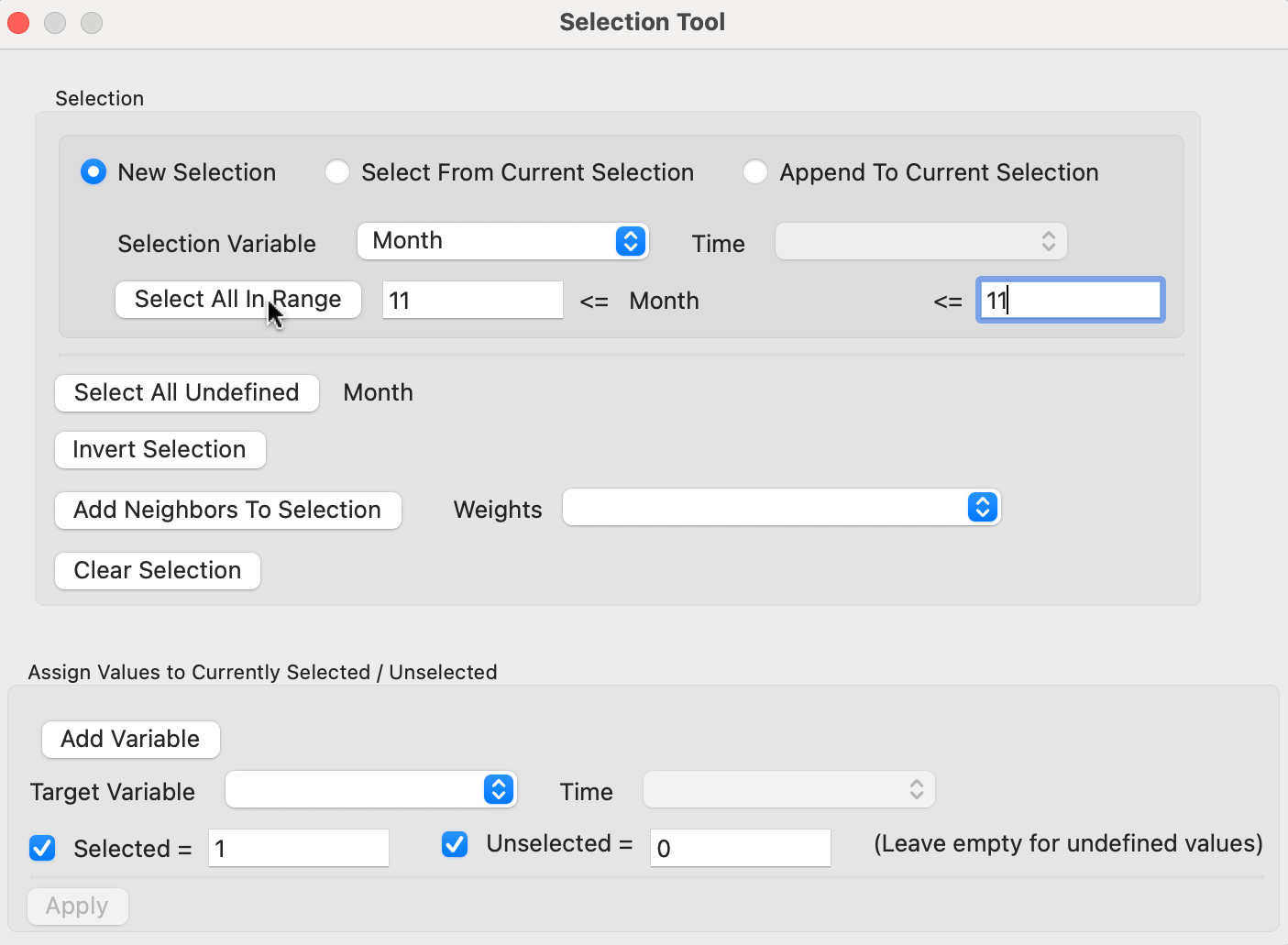
Figure 2.24: Selection Tool
2.5.1.1 New selection
The main panel of the interface deals with the selection criteria. In Figure 2.24, a New Selection has been started, as indicated by the radio button in the top line. To select the carjackings that occurred in the month of November, the Selection Variable must be set to the newly created variable Month. Also, the beginning and end value of the Select All in Range option must be set to 11 (for November). Clicking on the button will select the observations that meet the selection criterion.
The selected observations are immediately highlighted in the table. For clarity, they can also be moved to the top of the table by means of Table > Move Selected to Top. Simultaneously, the selected observations are also highlighted in the themeless point map. More precisely, they retain their original shading, while unselected observations become transparent.9
This is illustrated in Figure 2.25. The status bar lists that 207 observations have been selected. In addition, the selected observations are also immediately highlighted in any other open graph or map. This is the implementation of linking, which will be discussed in more detail in Chapter 4.
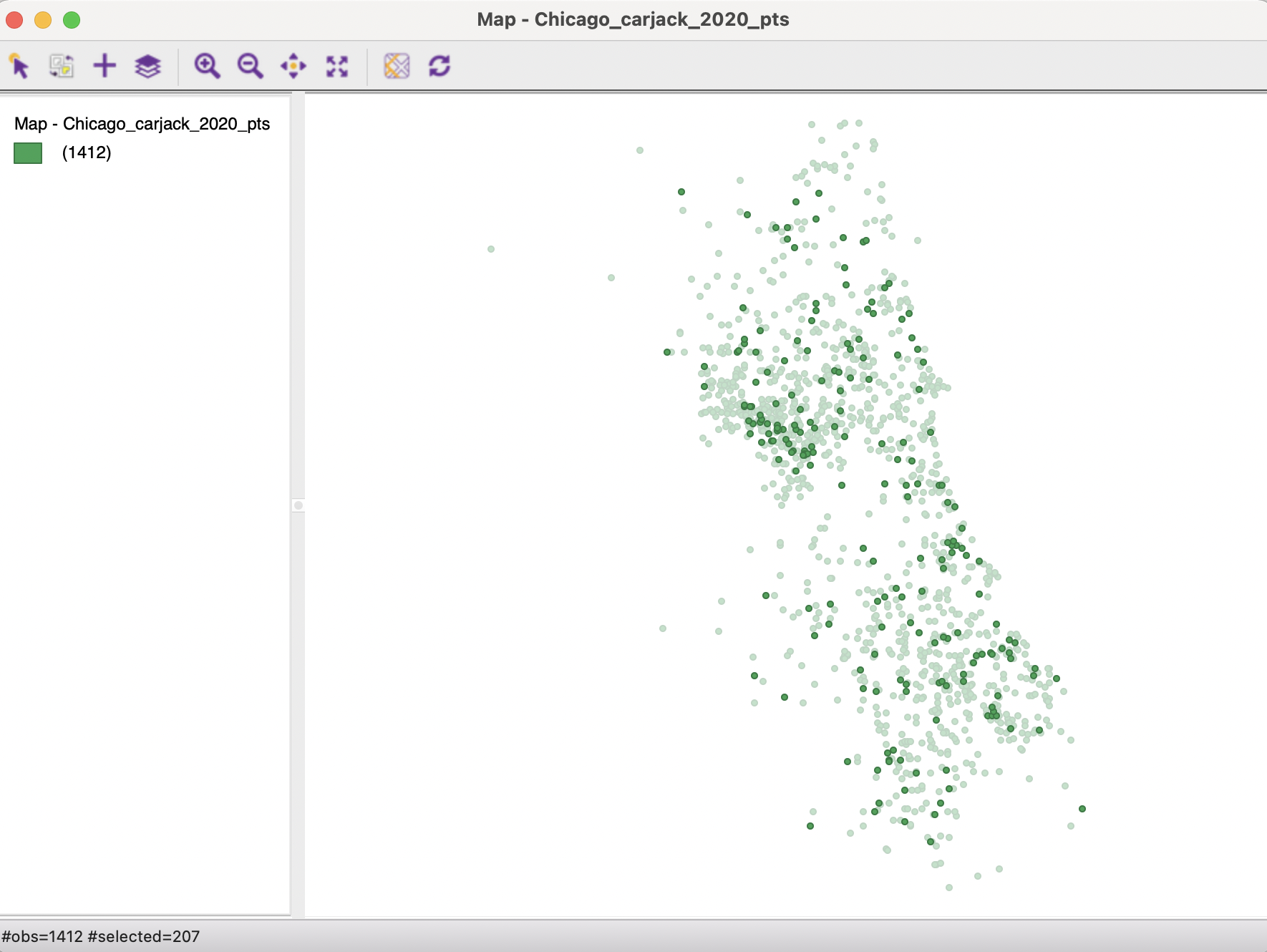
Figure 2.25: Selected observations in themeless map
2.5.1.2 Other selection options
The Selection Tool contains several more options to construct a more refined query. For example, a second criterion can be chosen to Select From Current Selection. This could be used to select a particular day of the month of November (provided the corresponding integer variable was created). Alternatively, to combine observations from both November and December, Append To Current Selection is appropriate.
A useful feature is to use Invert Selection to choose all observations except the selected ones. For example, this could be used to choose all months but November.
Often, this approach is the most practical way to remove unwanted observations, since there is no Save Unselected function. First, the observations to be removed are selected, followed by inverting the selection. At this point, File > Save Selected As can be employed to create a new data set (see Section 2.5.3).
The same approach can also be used in combination with Select All Undefined, which identifies the observations with missing values for a given variable. The inverted selection can then be saved as a data set without missing values.
The Add Neighbors To Selection option will be discussed in the chapters dealing with spatial weights, in Part III.
2.5.2 Indicator variable
Once observations are selected in the table, a new indicator variable can be created that typically holds the value of 1 for the selected observations, and 0 for the others, as shown in the bottom panel of Figure 2.24. More generally, any combination of values for presence/absence can be specified in the dialog.
With a Target Variable specified, clicking on Apply will add the 0-1 values to the table. This then makes the variable available for use as an indicator or conditioning variable in a range of statistical analyses, including conditional plots (covered in Volume 2) and analysis of variance.
2.5.3 Save selected observations
Arguably one of the most useful features of the selection tool in terms of data wrangling is the ability to save the selected observations as a new data set. This is accomplished by means of File > Save Selected As. For example, a new file can be specified to save just the observations for November, shown in Figure 2.26. The point pattern has the same shape as the selected observations in Figure 2.25, but the number of observations is now listed as 207.
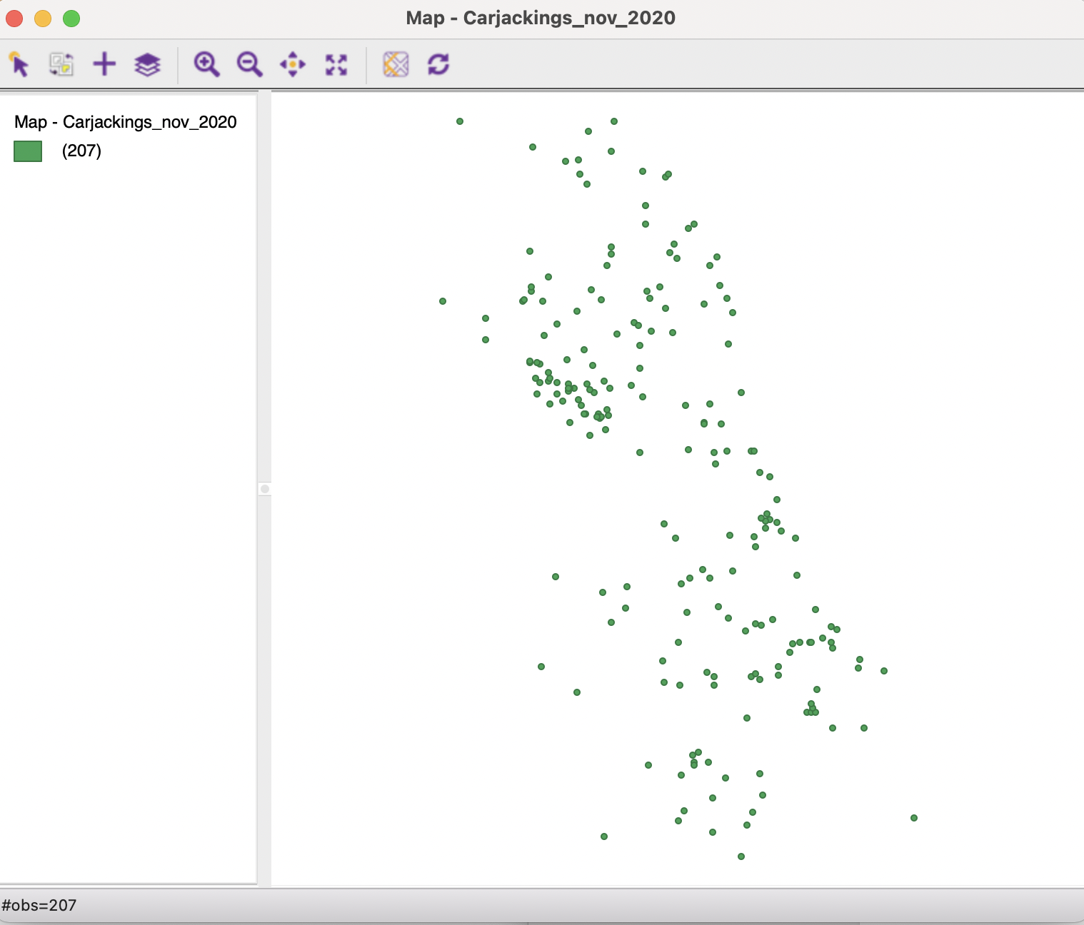
Figure 2.26: Selected observations in new map
2.5.4 Spatial selection
In addition to selecting observations by means of Table > Selection Tool, queries can also be constructed visually from any open map.
To illustrate the selection feature, a simple map of the points classified by month is shown in Figure 2.27.10 The number of observations in each category is listed next to the corresponding legend item, with (207) as the value for November.
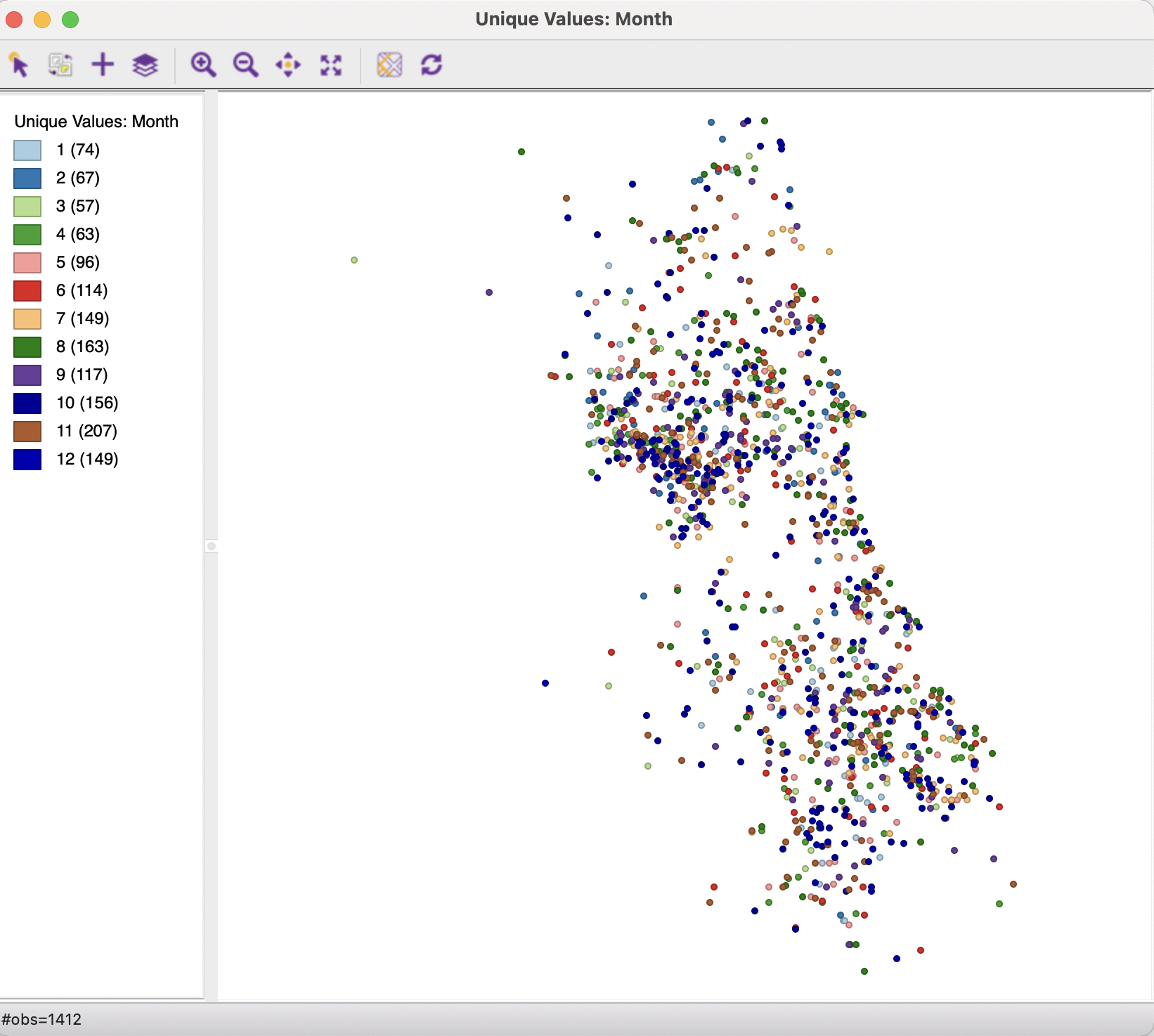
Figure 2.27: Car thefts by month
2.5.4.1 Selection by shape
The map selection tool – the pointer icon at the left of the map window toolbar – is the default interaction with a map view. Observations are selected by clicking on them or by drawing a selection shape around the target area. The default selection shape is a Rectangle, as in Figure 2.28, but Circle and Line are available as well. The particular shape is chosen by selecting Selection Shape from the map options menu (right click on the map).
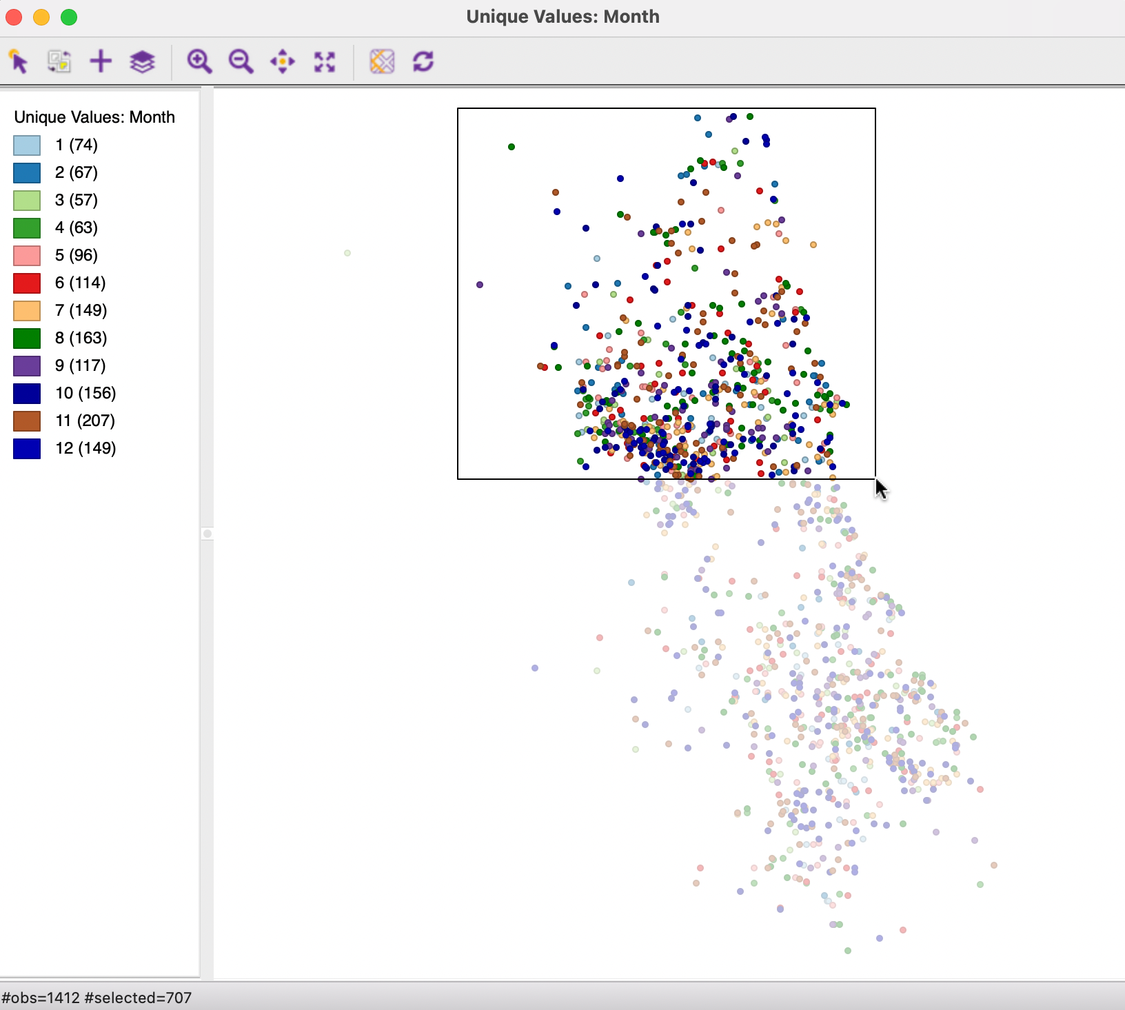
Figure 2.28: Selection on the map
Identical to table selection, all selected observations are highlighted in the table in yellow and in any other open map or graph (through linking). Also, they can be saved to a new data set using File > Save Selected As, in the same way as for a table selection.
The selection can be inverted by clicking on the second left-most icon in the map toolbar. This works in the same way as for table selection.
2.5.4.2 Selection on map classification
In addition to using a selection shape on a map, observations that fall into a particular map classification category can be selected by clicking on the corresponding legend icon. Map classifications are discussed in more detail in Chapter 4, but Figure 2.29 illustrates how the observations for the month November are selected by clicking on the small rectangle next to 11. The selected points match the pattern in Figure 2.25.
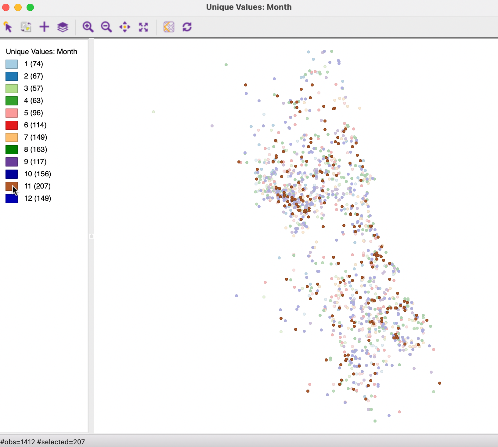
Figure 2.29: Selection on a map category
2.5.4.3 Save selection indicator variable
Finally, as is the case for a table selection, a new indicator variables can be saved to the table, with, by default, a value of 1 for the selected observations, and 0 for the others. This is invoked from the map options (right click on the map) by selecting Save Selection.
The default variable name is SELECTED, but this can be easily changed, as can the values assigned to selected and unselected. After the indicator variable is added to the table, it can be made permanent through a File > Save command, in the usual fashion.