8.3 Three Variables: Bubble Chart and 3-D Scatter Plot
When the number of dimensions is at most three, it remains relatively easy to visualize the multivariate attribute space. The bubble chart implements this by augmenting a standard two-dimensional scatter plot with an additional attribute for each point, i.e., the size of the point or bubble. More directly, observations can also be visualized as points in a three-dimensional scatter plot or data cube.
8.3.1 Bubble Chart
The bubble chart is an extension of the scatter plot to include a third and possibly a fourth variable into the two-dimensional chart. While the points in the scatter plot still show the association between the two variables on the axes, the size of the points, the bubble, is used to introduce a third variable. In addition, the color shading of the points can be used to consider a fourth variable as well, although this may stretch one’s perceptual abilities.
The introduction of the extra variable allows for the exploration of interaction. The point of departure (null hypothesis) is that there is no interaction. In the plot, this would be reflected by a seeming random distribution of the bubble sizes among the scatter plot points. On the other hand, if larger (or smaller) bubbles tend to be systematically located in particular subareas of the plot, this may suggest an interaction. Through the use of linking and brushing with the map, the extent to which systematic variation in the bubbles corresponds with particular spatial patterns can be readily investigated, in the same way as illustrated in the previous chapter.
The bubble chart was popularized through the well-known Gapminder web site, where it is
used extensively, especially to show changes over time.57 This aspect is currently
not implemented in GeoDa.
8.3.1.1 Implementation
The bubble chart is invoked from the menu as Explore > Bubble Chart, and from the toolbar by selecting the left-most icon in the multivariate group of the EDA functionality, shown in Figure 8.1. This brings up a Bubble Chart Variables dialog to select the variables for up to four dimensions: X-Axis, Y-Axis, Bubble Size and Bubble Color.
To illustrate this method, three variables from the Oaxaca Development sample data set are selected: peduc_20 (percent population with an educational gap in 2020) for the X-Axis, pserv_20 (percent population without access to basic services in the dwelling in 2020) for the Y-Axis, and pepov_20 (percent population living in extreme poverty in 2020) for both Bubble Size and Bubble Color. The default setting uses a standard deviational diverging legend (see also Section 5.2.3) and results in a somewhat unsightly graph, with circles that typically are too large, as in Figure 8.7.
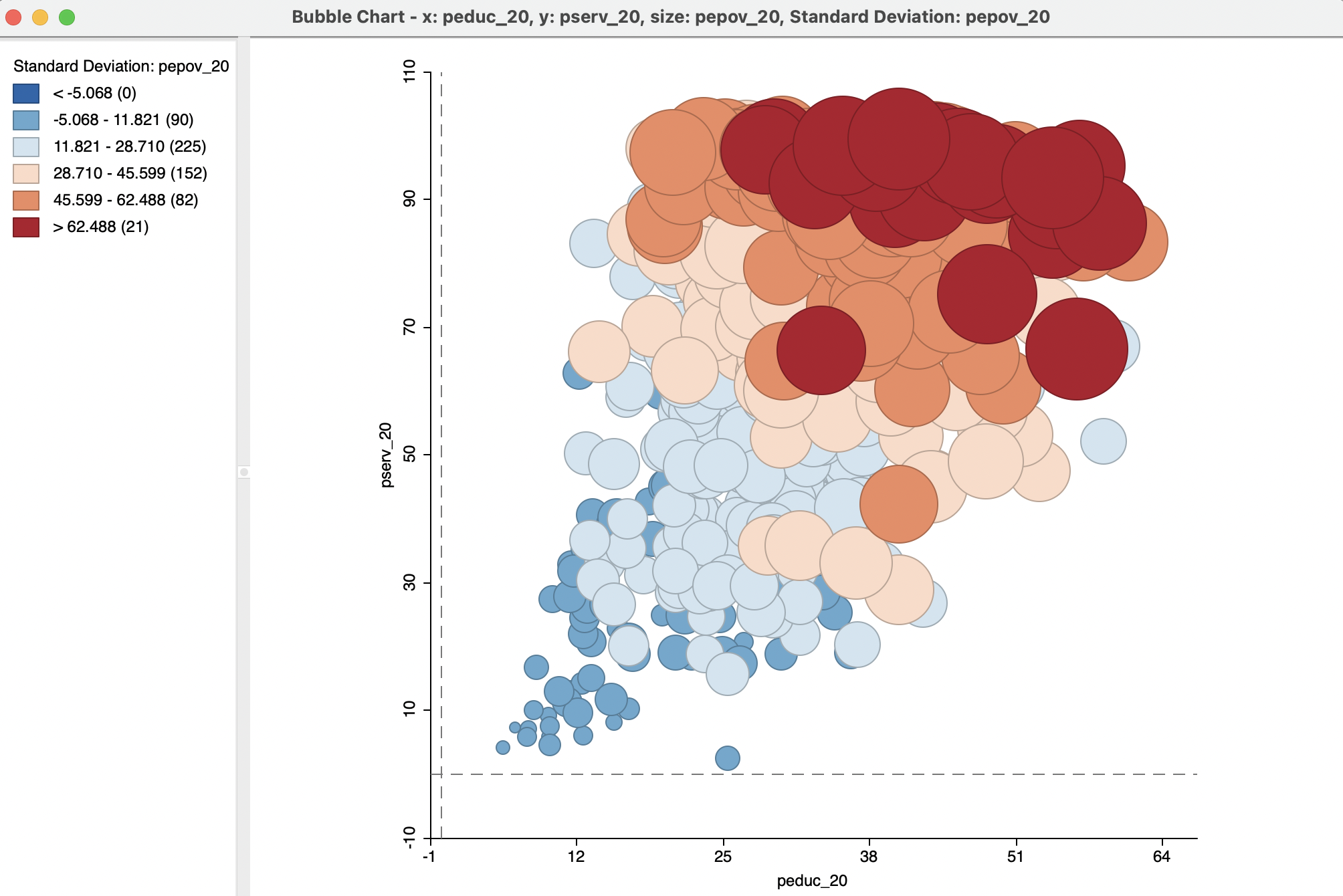
Figure 8.7: Bubble chart - default settings: education, basic services, extreme poverty
Before going into the options in more detail, it is useful to know that the size of the circle can be readily adjusted by means of the Adjust Bubble Size option. With the size significantly reduced, a more appealing Figure 8.8 is the result.
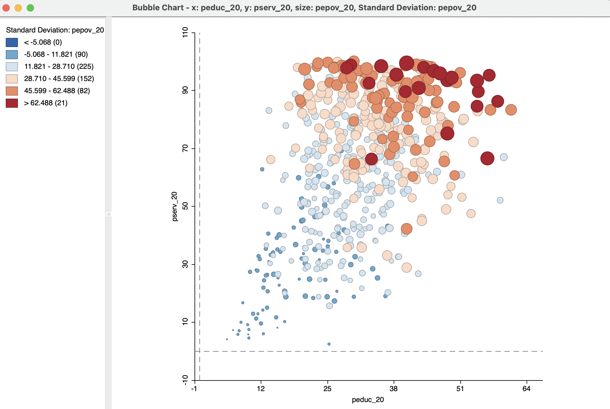
Figure 8.8: Bubble chart - bubble size adjusted: education, basic services, extreme poverty
As mentioned, the null hypothesis is that the size distribution (and matching colors) of the bubbles should be seemingly random throughout the chart. In the example, this is clearly not the case, with high values (dark brown colors and large circles) for pepov_20 being primarily located in the upper right quadrant of the graph, corresponding to low education and low services (high values correspond with deprivation). Similarly, low values (small circles and blue colors) tend to be located in the lower left quadrant. In other words, the three variables under consideration seem to be strongly related.
Given the screen real estate taken up by the circles in the bubble chart, this is a technique that lends itself well to applications for small to medium sized data sets. For larger size data sets, this particular graph is less appropriate.
8.3.1.2 Bubble chart options
In addition to Adjust Bubble Size, the bubble chart has nine main options, invoked in the usual fashion by right clicking on the graph. Several of these are shared with other graphs, in particular with the scatter plot, such as Save Selection, Copy Image To Clipboard, Save Image As, View, Show Status Bar and Selection Shape. They will not be further discussed here (see, e.g., Section 7.3.1). Classification Themes, Save Categories and Color work the same as for any map (see Section 4.5).
Figure 8.9 provides an illustration of the flexibility that these options provide. The graph pertains to the same three variables as before, but the Classification Themes option has been set to Themeless. As such, this results in green circles, but the Color option applied to the legend (see Section 4.5) allows the Opacity for the Fill Color for Category to be set to zero, resulting in the empty circles.
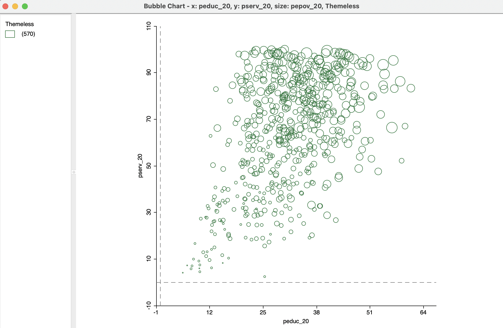
Figure 8.9: Bubble chart - no color: education, basic services, extreme poverty
8.3.1.3 Bubble chart with categorical variables
One particular useful feature to investigate potential structural change in the data is to use the Unique Values classification, in combination with setting the Size to a constant value.58
With peduc_20 for the X-Axis and ppov_20 (percentage population living in poverty) as the Y-Axis, Bubble Size is now set to the constant Const, with the categorical variable Region for Bubble Color.59 First, this yields a rather meaningless graph, based on the default standard deviation classification. Changing Classification Themes to Unique Values results in a scatter plot of the two variables of interest, with the bubble color corresponding to the values of the categorical variable. In the example, this is Region, as in Figure 8.10.
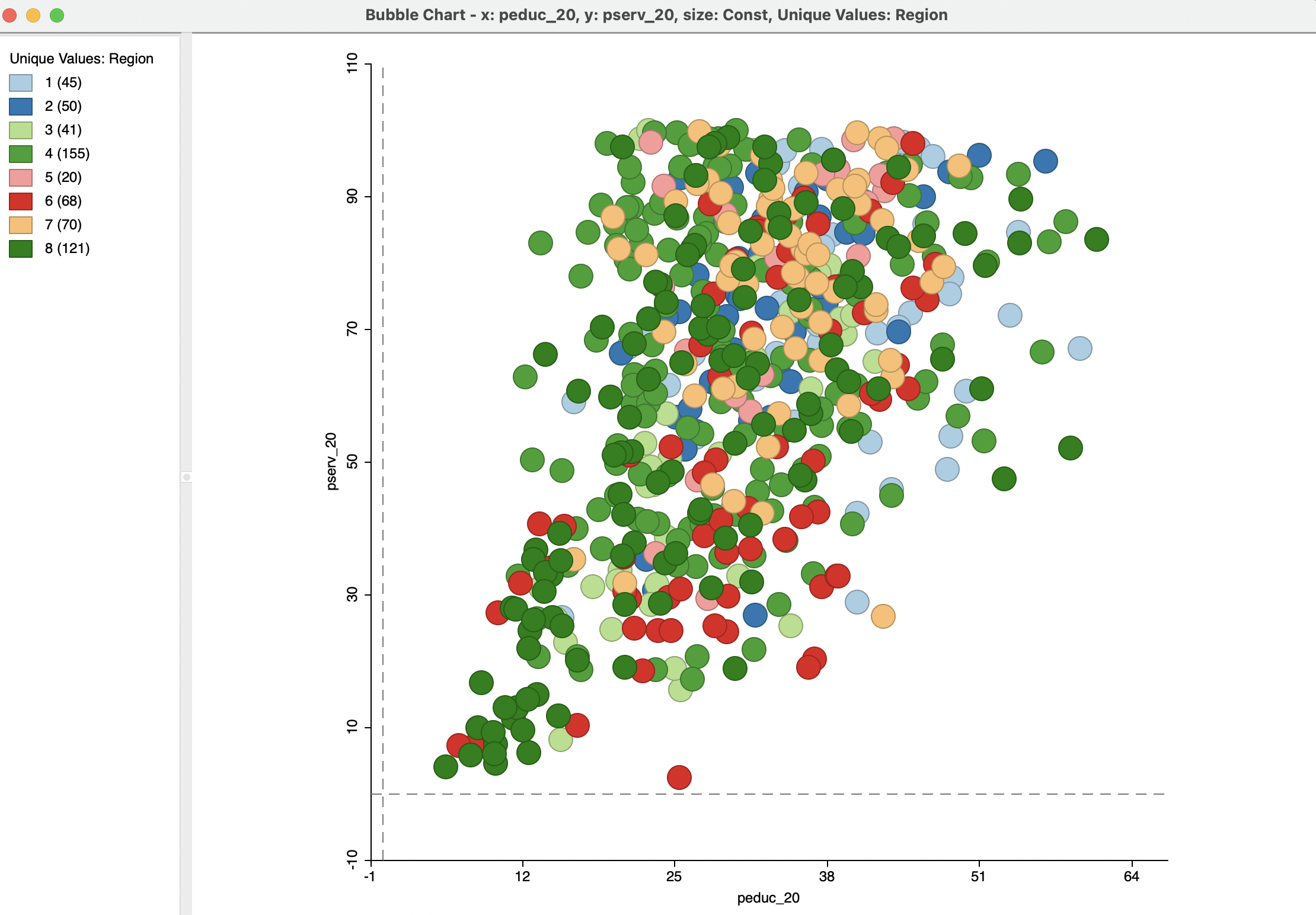
Figure 8.10: Bubble chart - categories: education, basic services, region
In this case, there seems to be little systematic variation along the region category, in line with our starting hypothesis.
The use of a bubble chart to address structural change is particularly effective when more than two categories are involved. In such an instance, the binary selected/unselected logic of scatter plot brushing no longer works. Using the bubble chart in this fashion allows for an investigation of structural changes in the bivariate relationship between two variables along multiple categories, each represented by a different color bubble. This forms an alternative to the conditional scatter plot, considered in Section 8.4.2.
8.3.2 3-D Scatter Plot
An explicit visualization of the relationship between three variables is possible in a three-dimensional scatter plot, the direct extension of principles used in two dimensions to a three-dimensional data cube. Each of the axes of the cube corresponds to a variable, and the observations are shown as a point cloud in three dimensions (of course, rendered as a perspective plot onto the two-dimensional plane of the screen).
The data cube can be manipulated by zooming in and out, in combination with rotation, to get a better sense of the alignment of the points in three-dimensional space. This takes some practice and is not necessarily that intuitive to many users. The main challenge is that points that seem close in the two-dimensional rendering on the screen may in fact be far apart in the actual data cube. Only by careful interaction can one get a proper sense of the alignment of the points.
8.3.2.1 Implementation
The three-dimensional scatter plot method is invoked as Explore > 3D Scatter Plot from the menu, or by selecting the second icon from the left on the toolbar depicted in Figure 8.1. This brings up a 3D Scatter Plot Variables selection dialog for the variables corresponding to the X, Y and Z dimensions. Again, peduc_20, pserv_20 and pepov_20 are used.
The corresponding initial default data cube is as in Figure 8.11, with the Y-axis (pserv_20) as vertical, and the X (peduc_20) and Z-axes (pepov_20) as horizontal. Note that the axis marker (e.g., the X etc.) is at the end of the axis, so that the origin is at the unmarked side, i.e., the lower left corner where the green, blue and purple axes meet.
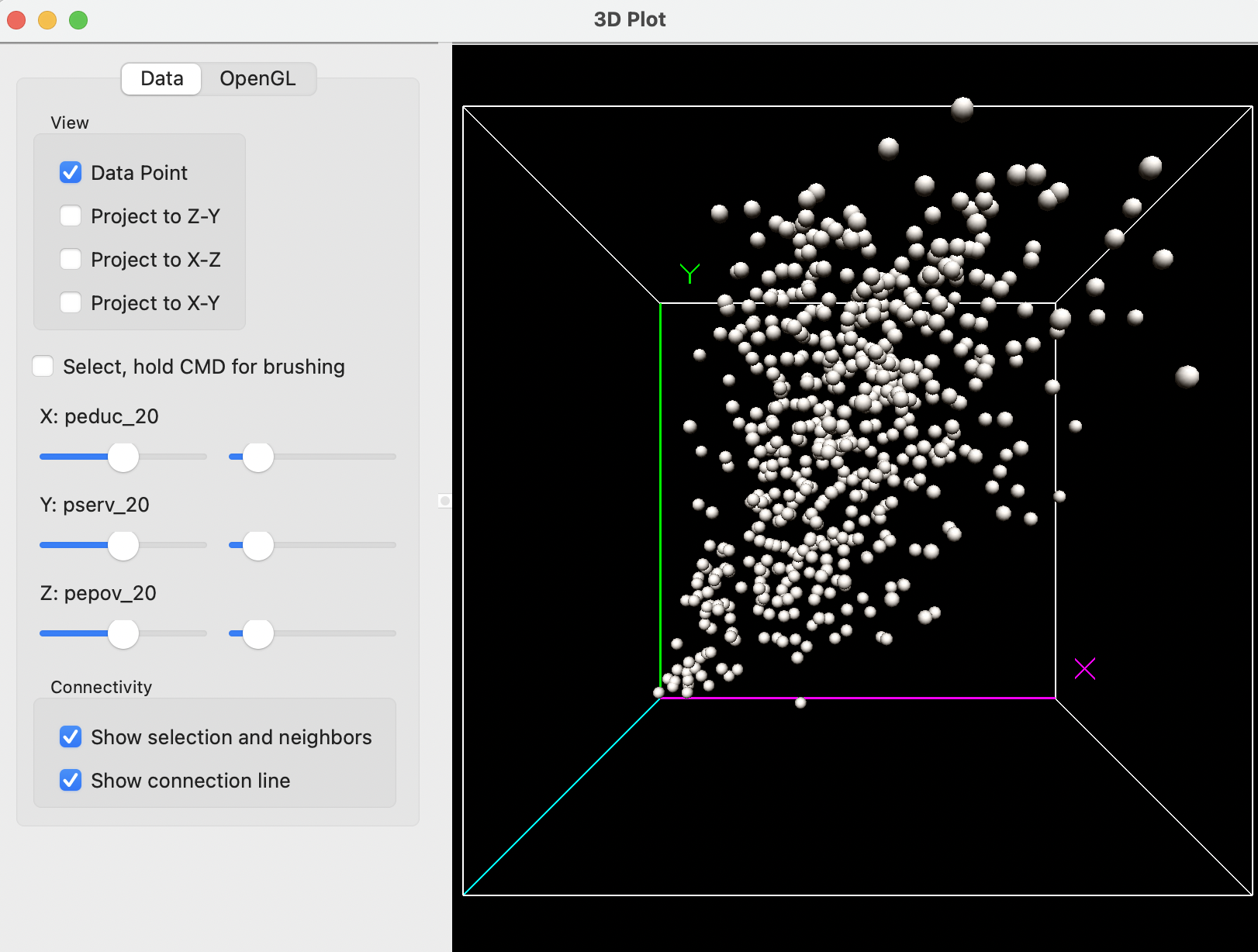
Figure 8.11: 3D scatter plot: education, basic services, extreme poverty
8.3.2.2 Interacting with the 3-D scatter plot
The data cube can be re-sized by zooming in and out. It is sometimes a bit ambiguous what is meant by these terms. For the purposes of this illustration, zooming out refers to making the cube smaller, and zooming in to making the cube larger (moving into the cube, so to speak).
The zoom functionality is carried out by pressing down on the track pad with two fingers and moving up (zoom out) or down (zoom in). Alternatively, one can press Control and press down on the track pad with one finger and move up or down. With a mouse, one moves the middle button up or down.
In addition, the cube can be rotated by means of the pointer: one can click anywhere in the window and drag the cube by moving the pointer to a different location. The controls on the left-hand side of the view allow for the projection of the point cloud onto any two-dimensional pane, and the construction of a selection box by checking the relevant boxes and/or moving the slider bar (see Section 8.3.2.3).
For example, in Figure 8.12, the cube has been zoomed out and the axes rotated such that Z is now vertical. With the Project to X-Y box checked on the left, a 2-dimensional scatter plot is projected onto the X-Y plane, i.e., showing the relationship between peduc_20 and pserv_20.
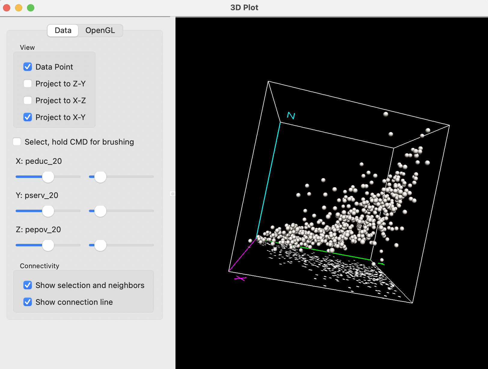
Figure 8.12: Interacting with 3D scatter plot
8.3.2.3 Selection in the 3-D scatter plot
Selection in the three dimensional plot (or, rather, its two-dimensional rendering) is a little tricky and takes some practice. The selection can be done either manually, by pressing down the command key while moving the pointer, or by using the guides under the Select, hold CMD for brushing check box.
Checking this box creates a small red selection cube in the graph. The selection cube can be moved around with the command key pressed, or can be moved and resized by using the controls to the left, next to X:, Y:, and Z:, with the corresponding variables listed.
The first set of controls (to the left) move the box along the matching dimension, e.g., up or down the X values for larger or smaller values of peduc_20, and the same for the other two variables. The slider to the right changes the size of the box in the corresponding dimension (e.g., larger along the X dimension). The combination of these controls moves the box around to select observation points, with the selected points colored yellow.
The most effective way to approach this is to combine moving around the selection box and rotating the cube. The reason for this is that the cube is in effect a perspective plot, and one cannot always judge exactly where the selection box is located in three-dimensional space.
A selection is illustrated in Figure 8.13, where only a few out of seemingly close points in the data cube are selected (yellow). By further rotating the plot, one can get a better sense of their location in the point cloud.
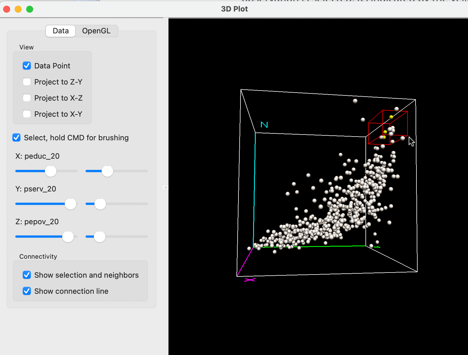
Figure 8.13: Selection in the 3D scatter plot
As in all other graphs, linking and brushing is implemented for the 3D scatter plot as well. Figure 8.14 shows an example of brushing in the six quantile map for ALTID and the associated selection in the point cloud. The assessment of the match between closeness in geographical space (the selection in the map) and closeness in multivariate attribute space (the point cloud) is a fundamental notion in the consideration of multivariate spatial correlation, discussed in Chapter 18.

Figure 8.14: Brushing and linking with the 3D scatter plot
Similar to the bubble chart, the 3D scatter plot is most useful for small to medium sized data sets. For larger numbers of observations, the point cloud quickly becomes overwhelming and is no longer effective for visualization.
8.3.2.4 3-D scatter options
The 3D scatter plot has a few specialized options, available either on the Data pane (which was considered exclusively so far), or on the OpenGL pane. The latter gives the option to adjust the Rendering quality of points, the Radius of points, as well as the Line width/thickness and Line color. These are fairly technical options that basically affect the quality of the graph and the speed by which it is updated. In most situations, the default settings are fine.
Finally, under the Data button, there are the Show selection and neighbors and Show connection line options. These items are relevant when a spatial weights matrix has been specified. This is covered in Chapter 10.
https://www.gapminder.org/tools/#$chart-type=bubbles&url=v1↩︎
A constant variable can be readily created by means of the Calculator option in the data table. Specifically, the Univariate tab with ASSIGN allows one to set the a variable equal to a constant.↩︎
The regional classifications are: (1) Canada; (2) Costa; (3) Istmo; (4) Mixteca; (5) Papaloapan; (6) Sierra Norte; (7) Sierra Sur; and (8) Valles Centrales.↩︎