14.3 Bivariate Spatial Correlation
The concept of bivariate spatial correlation is complex and often misinterpreted.
It is typically considered to be the correlation between one variable and the spatial
lag of another variable, as originally implemented in the precursor of GeoDa
(described in Anselin, Syabri, and Smirnov 2002). However, this formulation does not necessarily take into account
the inherent correlation between the two variables. More precisely, in a bivariate Moran’s I, the correlation is between \(x_i\) at location \(i\) and its neighbors \(\sum_j w_{ij} y_j\), where \(x\) and \(y\) are different variables. As formulated, this concept does not take into
account the correlation between \(x_i\) and \(y_i\), i.e., between the two variables at
the same location.
As a result, a bivariate Moran’s I statistic is often interpreted incorrectly, as it may overestimate the spatial aspect of the correlation that instead may be due mostly to the in-place correlation.104
14.3.1 Bivariate Moran scatter plot
In its initial conceptualization in Anselin, Syabri, and Smirnov (2002), a bivariate Moran scatter plot extends the idea of a Moran scatter plot with a variable on the horizontal axis and its spatial lag on the vertical axis to a bivariate context. The fundamental difference is that in the bivariate case the spatial lag pertains to a different variable. In essence, this notion of bivariate spatial correlation measures the degree to which the value for a given variable at a location is correlated with its neighbors for a different variable.
As in the univariate Moran scatter plot, the interest is in the slope of the linear fit to the scatter plot. This yields a Moran’s I-like statistic as: \[I_B = \frac{\sum_i (\sum_j w_{ij} y_j \times x_i)}{ \sum_i x_i^2},\] or, the slope of a regression of \(Wy\) on \(x\).
As before, all variables are expressed in standardized form, such that their means are zero and their variance one. In addition, the spatial weights are row-standardized.
Note that, unlike in the univariate autocorrelation case, the regression of \(x\) on \(Wy\) also yields an unbiased estimate of the slope, providing an alternative perspective on bivariate spatial correlation (see Section 14.4). In the case of the regression of \(x\) on \(Wx\), the explanatory variable \(Wx\) is endogenous, so that the ordinary least squares estimation of the linear fit is biased. However, with \(Wy\) referring to a different variable, the so-called simultaneous equation bias becomes a non-issue, and OLS in a regression of \(x\) on \(Wy\) has all the standard properties (such as unbiasedness).
A special case of bivariate spatial autocorrelation is when the variable is measured at two points in time, say \(z_{i,t}\) and \(z_{i,t-1}\), as in Section 14.2.1. The statistic then pertains to the extent to which the value observed at a location at a given time is correlated with its value at neighboring locations at a different point in time.
The natural interpretation of this concept is to relate \(z_{i,t}\) to \(\sum_j w_{ij} z_{j,t-1}\), i.e., the correlation between a value at \(t\) and its neighbors in a previous time period: \[I_T = \frac{\sum_i (\sum_j w_{ij} z_{j,t-1} \times z_{i,t})}{ \sum_i z_{i,t}^2},\] which expresses the effect of neighbors in \(t-1\) on the present value.
Alternatively, and maybe less intuitively, one can relate the value at a previous time period \(z_{t-1}\) to its neighbors in the future, \(\sum_j w_{ij} z_t\), as: \[I_T = \frac{\sum_i (\sum_j w_{ij} z_{j,t} \times z_{i,t-1})}{ \sum_i z_{i,t-1}^2},\] or the effect of a location at \(t-1\) on its neighbors in the future.
While formally correct, this may not be a proper interpretation of the dynamics involved. In fact, the notion of spatial correlation pertains to the effect of neighbors on a central location, not the other way around. While the Moran scatter plot seems to reverse this logic, this is purely a formalism, without any consequences in the univariate case. However, when relating the slope in the scatter plot to the dynamics of a process, this representation should be interpreted with caution.
A possible source of confusion is that the proper regression specification for a dynamic process would be as: \[z_{i,t} = \beta_1 \sum_j w_{ij} z_{j,t-1} + u_i,\] with \(u_i\) as the usual error term, and not as: \[z_{i,t-1} = \beta_2 \sum_j w_{ij} z_{j,t} + u_i,\] which would have the future predicting the past. This contrasts with the linear regression specification used (purely formally) to estimate the bivariate Moran’s I, for example: \[\sum_j w_{ij} z_{j,t-1} = \beta_3 z_{i,t} + u_i.\] In terms of the interpretation of a dynamic process, only \(\beta_1\) has intuitive appeal. However, in terms of measuring the degree of spatial correlation between past neighbors and a current value, as measured by the linear fit in a Moran scatter plot, \(\beta_3\) is the correct interpretation.
In the univariate case, only the specification with the spatially lagged variable on the left hand side yields a valid estimate. As a result, for the univariate Moran’s I, there is no ambiguity about which variables should be on the x-axis and y-axis. In contrast, in the bivariate case, both options are valid, although with a different interpretation.
Inference is again based on a permutation approach, but with an important difference. Since the interest focuses on the bivariate spatial association, the values for \(x\) and \(y\) are fixed at their locations, and only the remaining values for \(y\) are randomly permuted. In the usual manner, this yields a reference distribution for the statistic under the null hypothesis that the spatial arrangement of the remaining \(y\) values is random. It is important to keep in mind that since the focus is on the correlation between the \(x\) value at \(i\) and the \(y\) values at the neighboring locations, the correlation between \(x\) and \(y\) at location \(i\) is ignored.
14.3.1.1 Creating a bivariate Moran scatter plot
A bivariate Moran scatter plot is created as the second item in the drop down list activated by the Moran scatter plot toolbar icon (Figure 13.1). Alternatively, it can be started from the main menu as Space > Bivariate Moran’s I.
The variables and spatial weights are selected through the Bivariate Moran Variable Settings dialog. This allows for the selection of the First Variable (X), the Second Variable (Y), and the Weights from corresponding drop down lists. Since the version of the Oaxaca Development data set used here is time enabled, there are also drop down lists for the Time period.
To illustrate this functionality, the same variables are used as in Section 14.2.1, again with queen contiguity spatial weights (oaxaca_q). For the bivariate Moran’s I, the x-variable is then p_PHA (2020) and the y-variable its spatial lag in 2010, W_pPHA (2010).
The resulting graph is shown in Figure 14.6. The linear fit is almost horizontal, reflected by a Moran’s I of -0.008. Randomization, using 999 permutations, yields a pseudo p-value of 0.363, clearly not significant. This result may seem surprising, given the strong spatial autocorrelation found for p_PHA in each of the individual years (Figure 14.3). One possible explanation for this finding is that whereas there is strong evidence of clustering in each year, the location of the clusters may be different. Therefore, the relationship between the value at a given location and its neighbors in a different year may be weak, as is the case in this example.
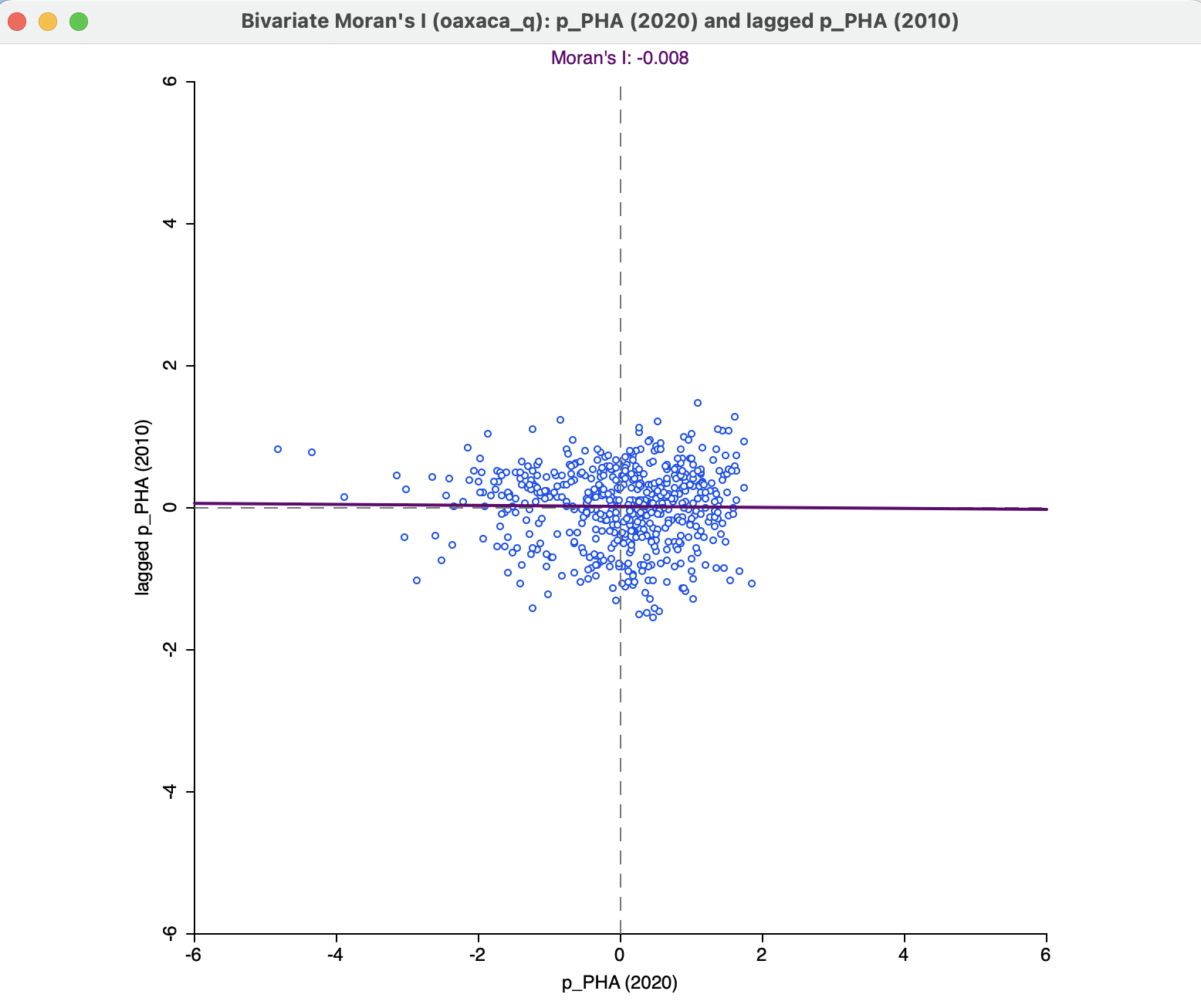
Figure 14.6: Bivariate Moran scatter plot for access to health care 2020 and its spatial lag in 2010
All the same options as for the univariate Moran scatter plot apply here as well. Also, the standardized value of the x variable and the spatial lag of the y-variable (applied to its standardized value) can be saved to the table, in the same way as for the univariate Moran scatter plot.