3.6 Multi-Layer Support
So far, the focus has been on a single spatial layer, associated with one cross-sectional data set. Over time, GeoDa has added some limited functionality to handle multiple layers, to facilitate operations such as a spatial join between two layers (see Section 3.7).
While multiple layers can be displayed in the same map window, interaction is limited to a single layer, the so-called current layer. This pertains to table manipulations, such as selection and variable transformation, but also to the full range of mapping and analytical functionality. The current layer is always the layer that was loaded first, irrespective of the actual order of the layers displayed in the map window.
Before delving deeper into the interaction between layers, the basics of the multiple layer logic in GeoDa are outlined.
3.6.1 Loading multiple layers
The starting point in any multi-layer operation is the current layer, i.e., the data set first loaded. For example, to display the carjacking locations together with the boundaries of the Chicago community areas, one of these layers must be the starting point, such as the points layer (shown Figure 2.7). An additional layer is loaded by means of the Add Map Layer option. This is represented by the large + icon, third from left in the map window toolbar.
This brings up the usual data input interface, to which the projected community area boundaries are loaded (e.g., community_areas_proj.shp, shown in Figure 3.4). The result is displayed in Figure 3.19, with the point locations portrayed on top of the community area outlines. The Map Layer Settings option (fourth icon from the left on the map window toolbar) brings up a small dialog that lists the order of the layers and indicates the current map.
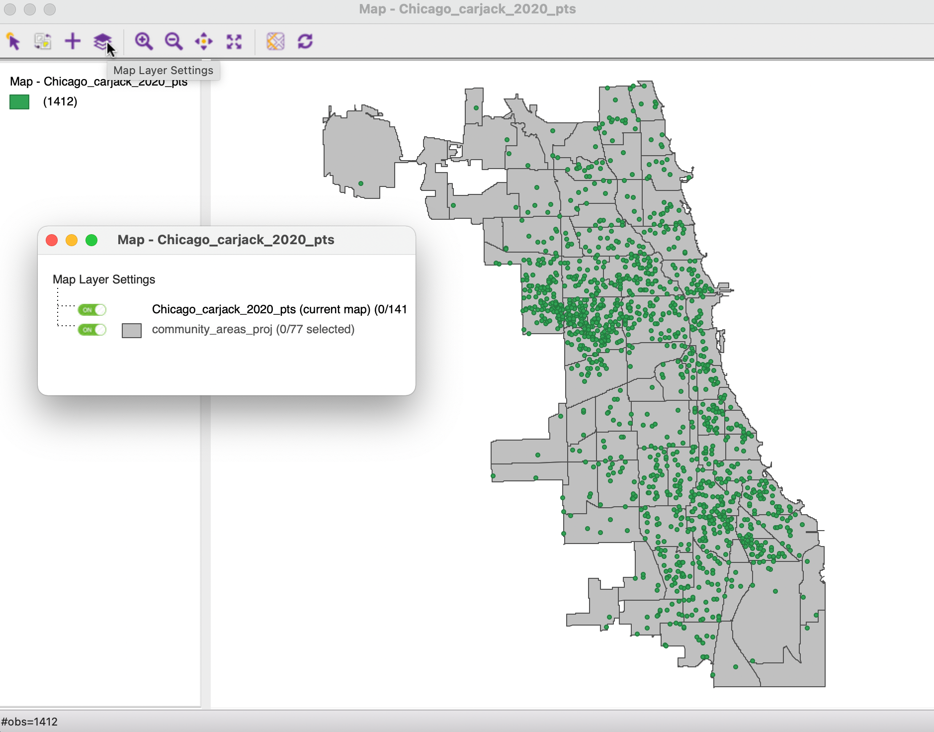
Figure 3.19: Map layer settings
It is important to keep in mind that the visual properties (such as color and opacity) of the current layer are managed by the map legend (see Chapter 4). The properties of the other layers are controlled through the Map Layer Settings.
3.6.1.1 Map layer setting options
A right click on the small legend rectangle associated with each layer (other than the current layer) brings up a list of options that pertain to the visual representation of that layer. The full list is shown in Figure 3.20.
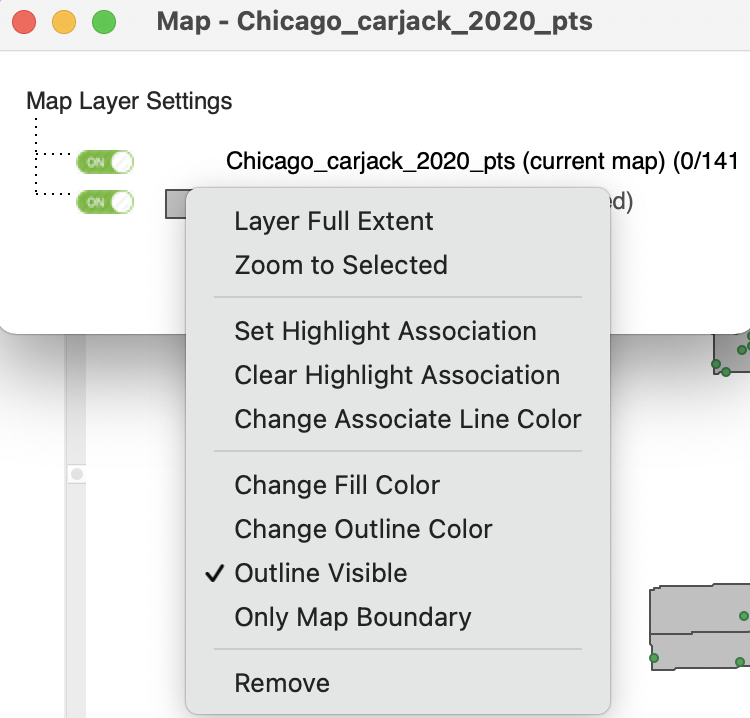
Figure 3.20: Customizing the second map layer
The two most often used functions are in the third set, i.e., Change Fill Color and Change Outline Color. In addition to setting the color, it may be necessary to adjust the opacity in order to make sure that the relevant information is visible. Specifically, setting opacity to 0 makes the areas invisible and only the boundary outlines are shown. The latter can be turned off by unchecking the Outline Visible option. The Only Map Boundary option results in a dissolve, in that only the outer outline of the polygon layer is shown. This operation is purely visual and does not involve any aggregation, in contrast to what was the case in Section 3.5.1.
The interface also includes options to set the association highlight, which is covered in Section 3.8. The final item in the dialog is to Remove the layer.21
3.6.1.2 Layer position
The position of the layers in the map view can be altered by means of the Map Layer Settings interface. One grabs the entry for a layer and drags it to a different position. For example, in Figure 3.21, the community area layer is moved to the top (this requires setting the opacity to 0 in order for the points to show). However, even though the polygon layer is now on top, the point layer remains the current map layer, since it was loaded first.
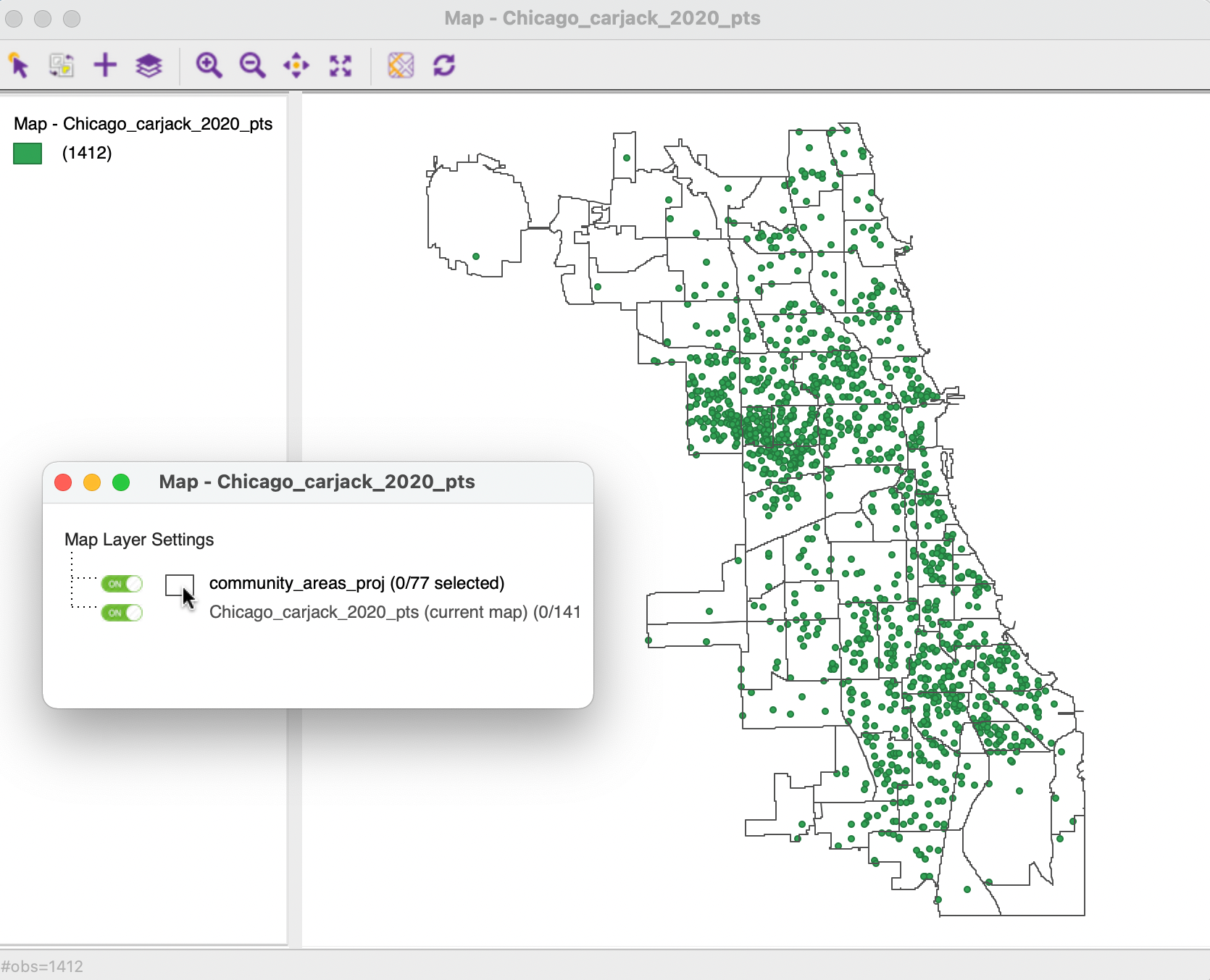
Figure 3.21: Polygon layer on top with opacity=0
3.6.2 Automatic reprojection
In the previous example in Figure 3.19, the two layers that combined were expressed in the same projection. More precisely, the projected community area boundaries were superimposed on the point layer.
However, as long as layers have projection information associated with them, any added layer will be reprojected to the projection of the current layer. This is for visualization only, and it does not change the projection information in the files of the reprojected layers.
For example, in Figure 3.22, the order in which the layers are loaded is reversed from Figure 3.19. The community area layer (Chicago_community_areas.shp) is loaded first (i.e., it is the current layer). This layer is not projected, but expressed in lat-lon coordinates. To this the point layer Chicago_carjack_2020_pts.shp is added, which is projected.
Initially, the point layer is invisible, since it is positioned under the polygon layer. The default green coloring of the community areas masks the points underneath. After setting the opacity of the top layer to zero, the points become visible.
In Figure 3.22, a slightly more spread out pattern can be noticed relative to Figure 3.19. Under the hood, the point layer has been reprojected to lat-lon decimal degrees. This is only for visualization in the map view, and does not change the CRS associated with the added layers.
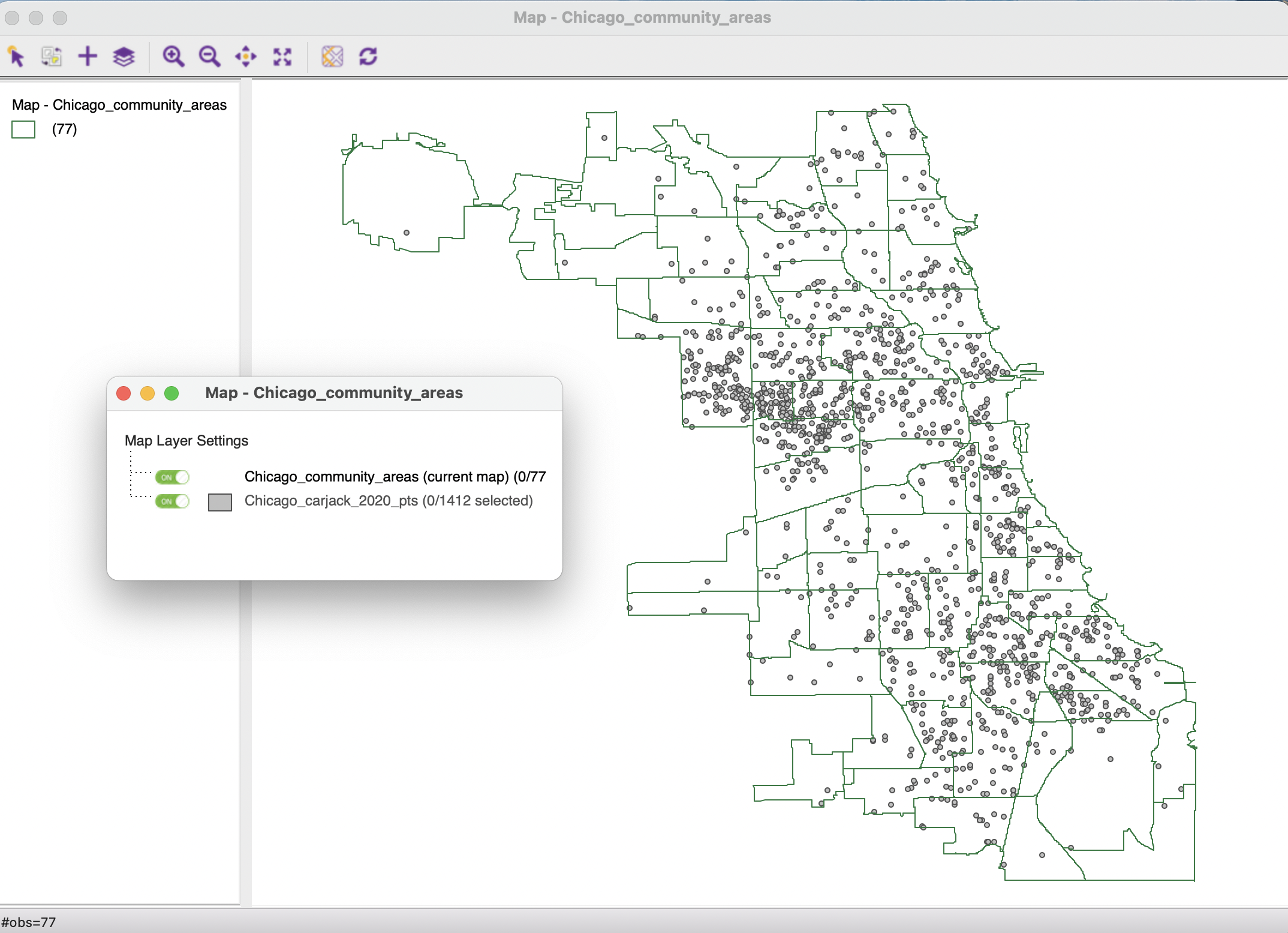
Figure 3.22: Points reprojected to lat-lon
3.6.3 Selection in multiple layers
It is important to keep in mind that any selection only pertains to the current map layer, which may or may not also be the top layer. For example, continuing with the previous illustration (Figure 3.22), any selection will pertain to the community area layer, which is the current map layer. This is irrespective of which layer is shown as the top layer.
In Figure 3.23, the selection status bar indicates that 14 observations were selected. If the point layer was moved to the top, this would give the same result.
This logic may seem a bit counter-intuitive at first, but it is based on the linking and brushing architecture implemented
in GeoDa (see Chapters 4 and 7 for a more extensive discussion). Currently, the linking operation works only for a single layer, which is always the first loaded layer.
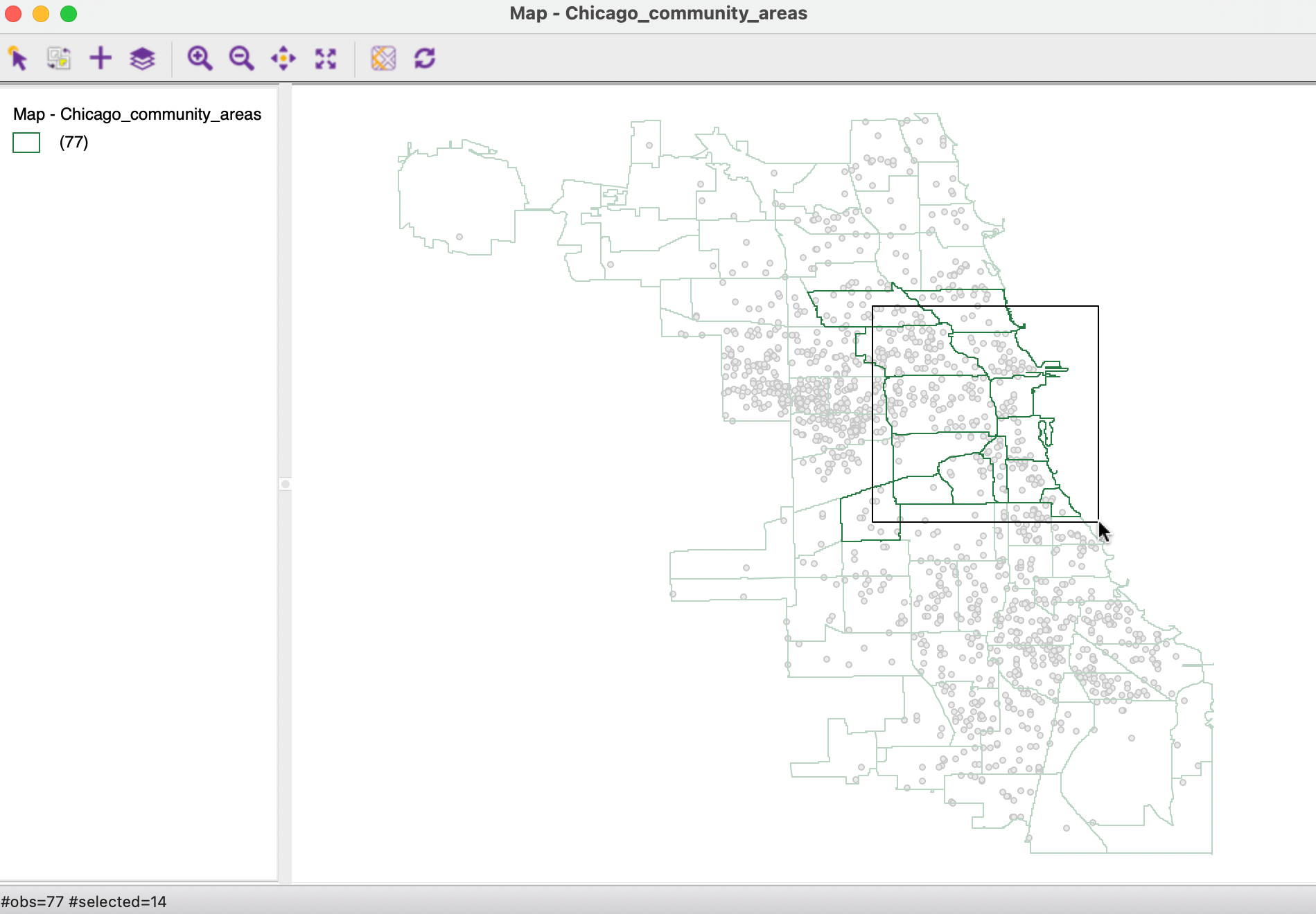
Figure 3.23: Select on current map layer (community areas)
In addition, it is possible to change the map window scope by using Zoom to Selected and Layer Full Extent.↩︎