11.4 Implementation
As mentioned in the chapter introduction, the distance-based weights functionality is illustrated with a point layer of 261 Italian community banks, shown in Figure 11.2.77
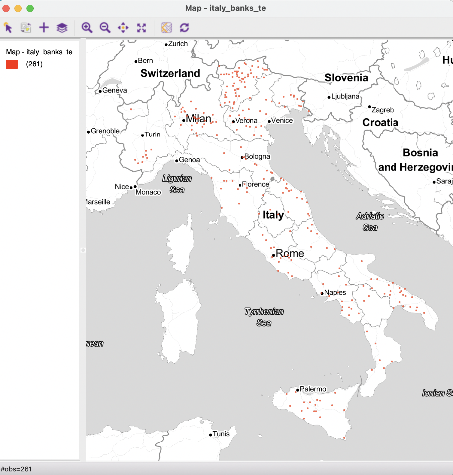
Figure 11.2: Italian community bank point layer
Distance weights are invoked in the same way as contiguity weights, through the Weights Manager, as outlined in Section 10.3.1. The Weights File Creation dialog with the Distance Weight button selected is shown in Figure 11.3. The ID Variable is set to idd.
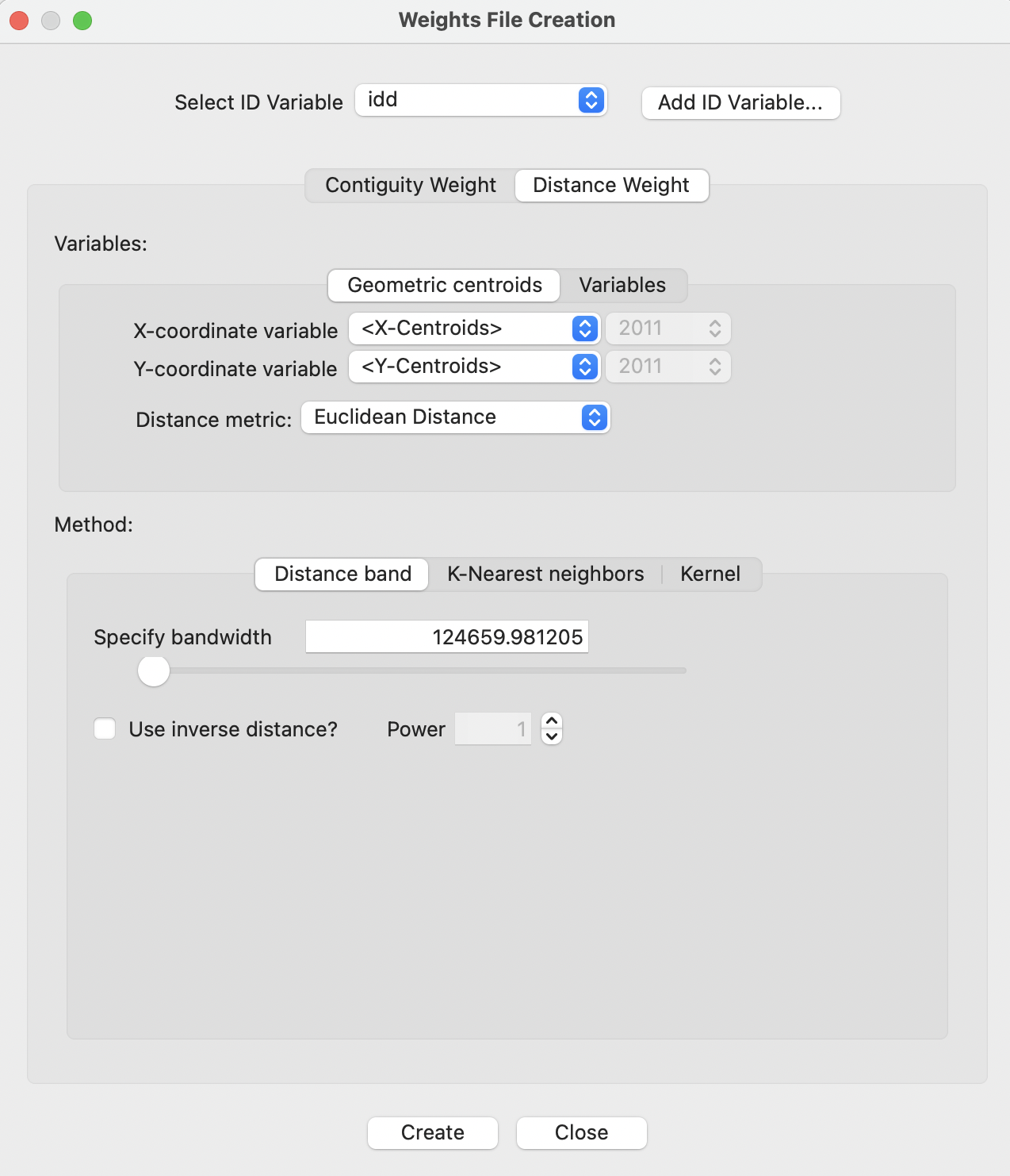
Figure 11.3: Distance-based weights in the Weights File Creation interface
The dialog controls the various options available to create distance-based weights. These include the choice between geographic distance - the Geometric centroids button under Variables - or generalized distance - the Variables button (see Section 11.4.4).
The default for geographic distances is to have the X-coordinate variable as the internally obtained X-Centroids, and the Y-coordinate variable as the internally obtained Y-Centroids. However, any other pair of variables can be selected, including non-geographic ones. The resulting concept of general distance is limited to two dimensions, whereas the Variables tab allows for higher dimensions as well.
The default Distance metric is Euclidean Distance. Other options, appropriate for unprojected coordinates, are Arc Distance (mi) and Arc Distance (km), for great circle distance expressed as either miles or kilometers.
The type of weight is set by the Method tab. The Distance band criterion is the default. Other options are K-Nearest neighbors and Kernel weights.78 The default bandwidth for distance band weights is the max-min distance. In the current example, this is listed as about 125 km (the units are meters). The options for inverse distance and Power are considered in Chapter 12.
11.4.1 Distance-band weights
With the default settings as in Figure 11.3, invoking Create will bring up the familiar file save dialog. As was suggested for contiguity weights, it is useful to make the file name reflect the nature of the weights since there are no metadata, unless a project file is created. In this example, the file name is italy_banks_te_d with the GWT file extension added automatically.
Once the file is created, it appears in the Weights Manager, as shown in Figure 11.4.
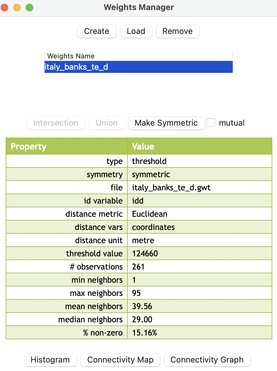
Figure 11.4: Default distance-based weights summary properties
The summary properties indicate the type as threshold, with threshold value as 124660, distance metric as Euclidean, distance vars as coordinates, and distance unit as meter. The other properties are the same as for contiguity weights (see Section 10.4.1).
Note how the range of the neighbor cardinality is much larger than for contiguity, going from 1 to 95. This reflects the impact of the max-min default cut-off distances on densely distributed points. The distance of about 125 km is much larger than the average distance that separates the community banks.
11.4.1.1 GWT file
Distance-based weights are saved in files with a GWT file extension. This format,
illustrated in Figure 11.5, is slightly different from the GAL format used for contiguity weights. It was first introduced in SpaceStat in 1995, and later adopted by R spdep and other software packages. The header line is the same as for GAL files, but each pair of neighbors is listed, with the ID of the observation, the ID of its neighbor and the distance that separates them.
The pairwise distance is currently only included for informational purposes, since GeoDa does not use the actual distance value in any statistical operations. In other words, the weights are turned into binary form and row-standardized by default. The only place where the distances are taken into account is in the computation of distance functions, covered in Chapter 12.
Note how observation with idd=1 has no less than 28 neighbors, with inter-point distances ranging from slightly over 20 km to almost 125 km.
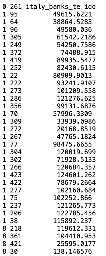
Figure 11.5: GWT weights file format
11.4.1.2 Weights characteristics
In the same way as for contiguity weights, the characteristics of distance-based weights can be assessed by means of the Connectivity Histogram, the Connectivity Map, and the Connectivity Graph. These are available through the buttons at the bottom of the weights manager.
The shape of the connectivity histogram for distance-band weights is typically very different from that of contiguity-based weights. As illustrated in Figure 11.6, the range in the neighbor cardinality is much larger than for contiguity weights. The distribution also includes extremes, with one observation having only one neighbor, and one having 95.
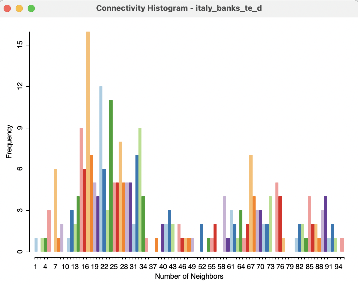
Figure 11.6: Connectivity histogram for default distance weights
As mentioned, the range in the number of neighbors is directly related to the density of the spatial distribution of the points. Locations that are somewhat isolated will drive the determination of the largest nearest neighbor cut-off point (their nearest neighbor distance will be large), whereas dense clusters of locations will encompass many neighbors using this large cut-off distance.
The properties of the distance band weights can be further investigated by means of the Connectivity Graph. As before, this is invoked through the right-most button at the bottom of the weights manager.
The pattern shown in Figure 11.7 highlights how the connectivity is highly uneven, with very dense areas alternating with much sparser distributions. The connection highlighted in blue corresponds to the max-min distance. Clearly, this distance is much larger than the average distance among locations, leading to a highly unbalanced weights matrix.
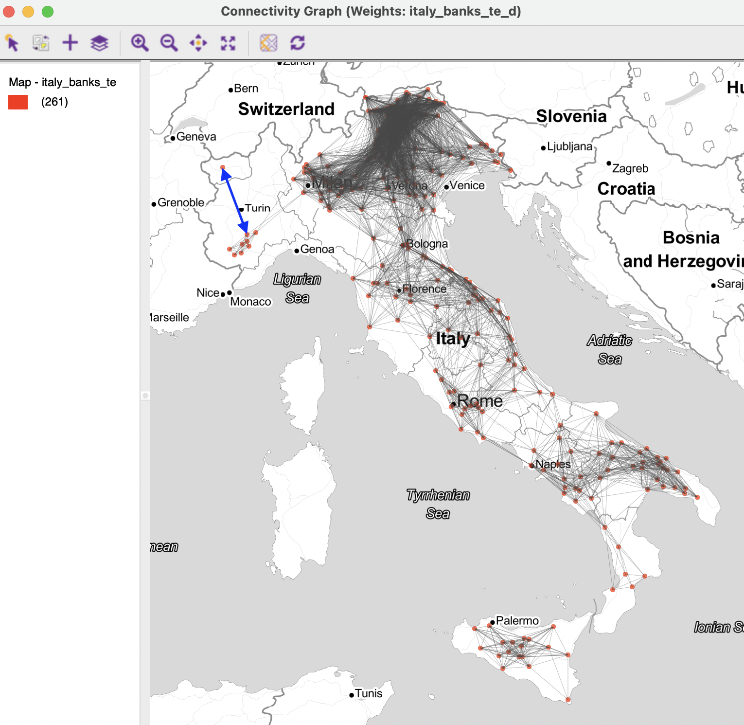
Figure 11.7: Connectivity graph for default distance weights
11.4.2 Isolates
The default distance band ensures that each observation has at least one neighbor, but this has several undesirable side effects. To create a more balanced weights matrix, one can lower the distance threshold. However, this will result in observations that do not have neighbors, isolates or islands.
The Weights File Creation dialog is flexible enough that a specific distance cut-off can be entered in the box, or the movable button can be dragged to any value larger than the minimum distance, but smaller than the max-min distance. Sometimes, theoretical or policy considerations suggest a specific value for the cut-off that may be smaller than the max-min distance.
When such a threshold is chosen, a warning will appear, pointing out that the specified cut-off value is smaller than the distance needed to ensure that each observation has at least one neighbor.
For example, using a cut-off distance of 73 km instead of the default 125 km yields a much sparser weights matrix (italy_banks_te_d73.gwt), as evidenced by the summary in Figure 11.8. The maximum number of neighbors has been reduced from 95 to 59 (which is still quite large), but, more importantly, the min neighbors is listed as 0. Compared to the default, the density has decreased substantially, going from 15.16 % non-zero elements to 7.87 % non-zero.
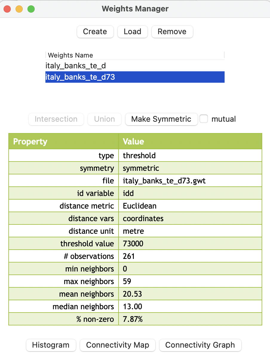
Figure 11.8: Weights summary properties for distance 73km
The connectivity graph shown in Figure 11.9 illustrates the greater sparsity. As it turns out, the distance band of 73 km resulted in only two isolates, highlighted in the figure, one near Aosta, in the north-west, and a second on the island of Sicily. All other observations are connected. However, there begin to form disconnected entities, i.e., separate components in the graph that are connected internally, but not between them.
Further lowering the cut-off distance may result in more meaningful groupings, but at the expense of a growing number of isolates.
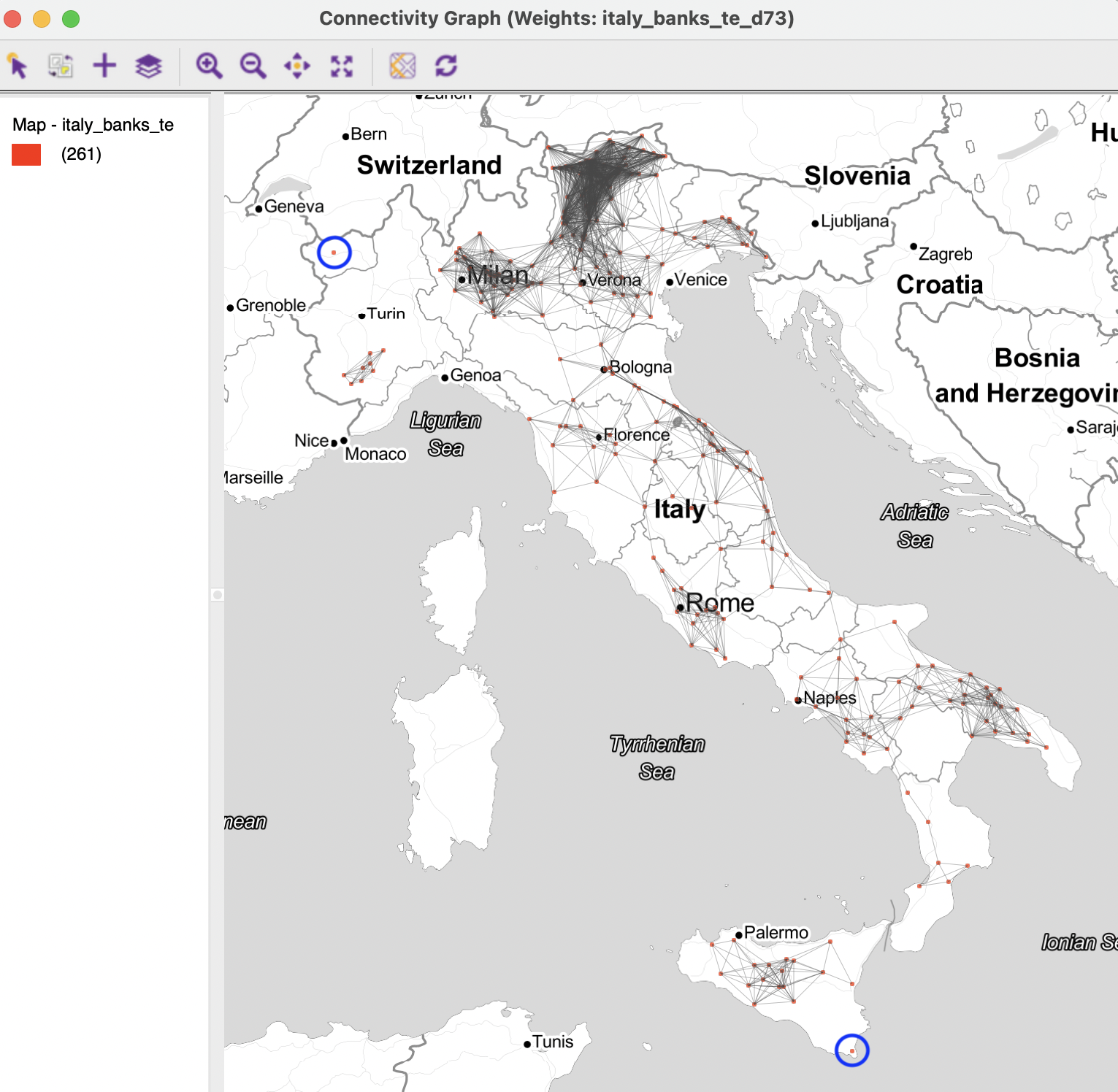
Figure 11.9: Connectivity graph for distance band 73km
11.4.2.1 How to deal with isolates
Since the isolated observations are not included in the spatial weights (in effect, the corresponding row in the spatial weights matrix consists of zeros), they are not accounted for in any spatial analysis, such as tests for spatial autocorrelation, or spatial regression. For all practical purposes, they should be removed from such analysis. However, they are fine to be included in a traditional non-spatial data analysis.
Ignoring isolates may cause problems in the calculation of spatially lagged variables, or measures of local spatial autocorrelation. By construction, the spatially lagged variable will be zero, which may suggest spurious correlations.
11.4.3 K-nearest neighbor weights
K-nearest neighbor (KNN) weights are computed by selecting the corresponding button in Distance Weight panel of the Weights File Creation interface. The value for the Number of neighbors (k) is the only option. The default is 4, but 6 is used in the example (as in Algeri et al. 2022).
The weights (saved as the file italy_banks_te_k6.gwt) are added to the collection contained in the weights manager. In addition, all its properties are listed, as illustrated in Figure 11.10. Note that the properties now include the number of neighbors instead of the distance threshold value, as was the case of distance-band weights. Also, symmetry is set to asymmetric, which is a fundamental difference with distance-band weights.
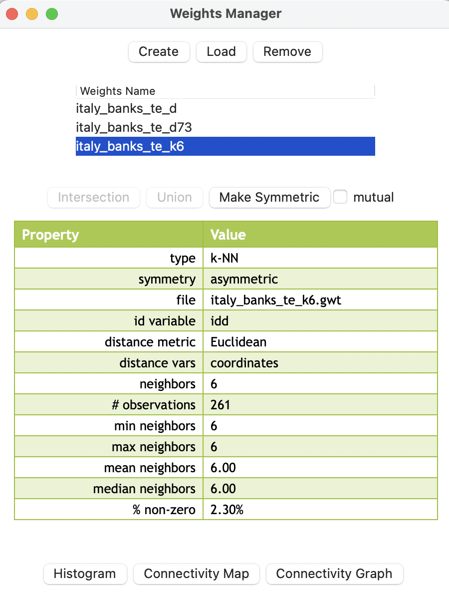
Figure 11.10: Weights summary properties for 6 k nearest neighbors
The properties listed in the weights manager also include the mean and median number of neighbors, which of course equal k (in the example, they equal 6). The resulting weights matrix is dramatically less dense relative to the distance-band weights (2.30% compared to 15.16%).
K-nearest neighbors weights are often an alternative when a realistic distance band results in too many isolates, since each observation has k neighbors by design. However, this approach is not without some drawbacks and may not be appropriate in all situations.
11.4.3.1 Weights characteristics
Again, the connectivity histogram, map and graph can be used to inspect the neighbor characteristics of the observations. However, in this case, the histogram doesn’t make much sense, since all observations have the same number of neighbors (by construction).
In contrast, the connectivity graph, shown in Figure 11.11, clearly demonstrates how each point is connected to six other points. In the example, this yields a fully connected graph.
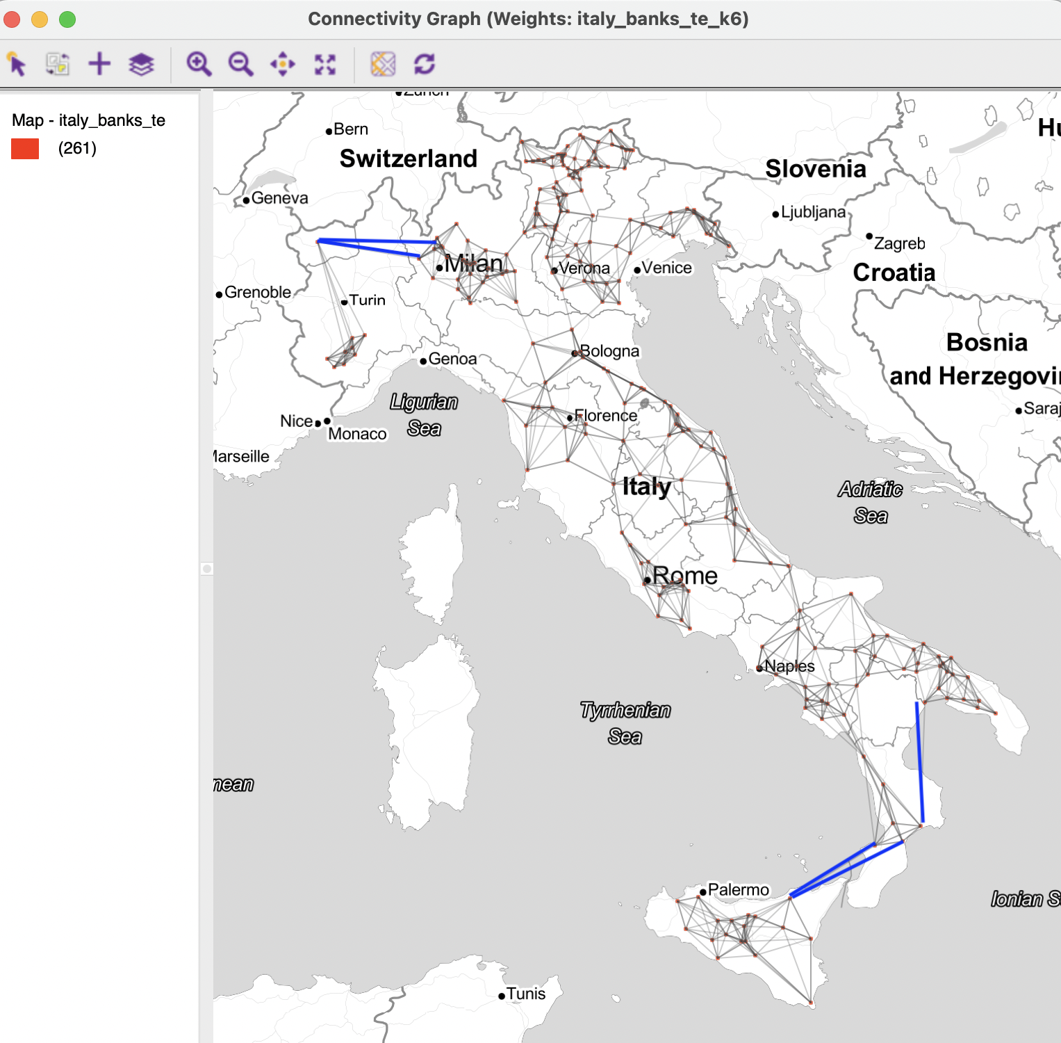
Figure 11.11: Connectivity graph for 6 k-nearest neighbors
11.4.3.2 Caveat
One drawback of the k-nearest neighbor approach is that it ignores the distances involved. The first k neighbors are selected, irrespective of how near or how far they may be. This suggests a notion of distance decay that is not absolute, but relative, in the sense of intervening opportunities (e.g., one considers the two closest grocery stores, irrespective of how far they may be).
In addition, the requirement to have exactly k neighbors may create artificial connections, spanning large distances or bridging across natural and other barriers. For example, in the graph in Figure 11.11, the blue lines highlight some instances where this is the case. In the case of the northern isolate, the Aosta location becomes connected to observations located near Milan. For an observation on the north coast of Sicily, two long connections are included across the straight of Messina to the boot of Italy. A similar distant neighbor is identified for a location in Calabria to a far away one in the region of Basilicata. It is unlikely that these connections correspond with meaningful interactions among the community banks.
The relative distance effect should be kept in mind before mechanically applying a k-nearest neighbor criterion.
11.4.4 General distance matrix
The Variables tab in the distance weights dialog (Figure 11.3) also allows for the computation of a general weights matrix. This is based on the distance between observations in multi-attribute space. Instead of selections for the X and Y coordinates, a drop-down list with all the variables is available. From this, any number of variables can be selected, not just two, as in the standard distance case.
In addition, there is a Transformation option that allows the usual standardizations (see Section 2.4.2.3). The distance metric can be either Euclidean Distance or Manhattan Distance (great circle distance is not meaningful in this context).
Typically, the variables are first standardized, such that their mean is zero and variance one, which is the default setting.
All the standard options are available, such as specifying a distance band (in multi-attribute distance units) or k-nearest neighbors. Such a general distance matrix or dissimilarity matrix is a required input in the multivariate clustering methods considered in Volume 2.