2.4 Table Manipulations
A range of variable transformations is supported through the Table functionality. This requires that the data table associated with a spatial layer is open. In contrast to the other operations in GeoDa, opening a
data table can
only be accomplished by selecting a toolbar icon, i.e.,
the second icon from right on the toolbar shown in Figure 2.1.
With the table open, the options can be accessed from the menu, by selecting the Table menu item, or by right clicking on the table itself. This brings up the list shown in Figure 2.16.
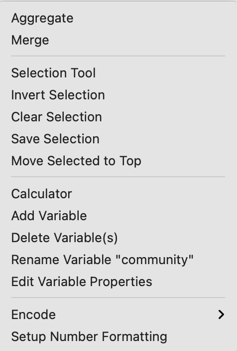
Figure 2.16: Table options
In addition to a range of variable transformations, the options menu also includes the Selection Tool, which is the way in which data queries can be carried out. I discuss this in more detail in Section 2.5. The more commonly used variable manipulations are covered in what follows.
2.4.1 Variable properties
2.4.1.1 Edit variable properties
One of the most used initial transformations pertains to getting the data into the right format. Often, observation identifiers, such as the FIPS code used by the U.S. census, are recorded as character or string variables. In order to use these variables effectively as observation identifiers, they need to be converted to a numeric format. This is accomplished through the Edit Variable Properties option.
After this option is invoked by clicking on it, a window appears with a list of all variables, listing their type, as well as a number of other properties, like precision.
For example, consider the data table associated with the Chicago_community_areas community area boundaries, shown in Figure 2.17, after selecting the Edit Variable Properties option.
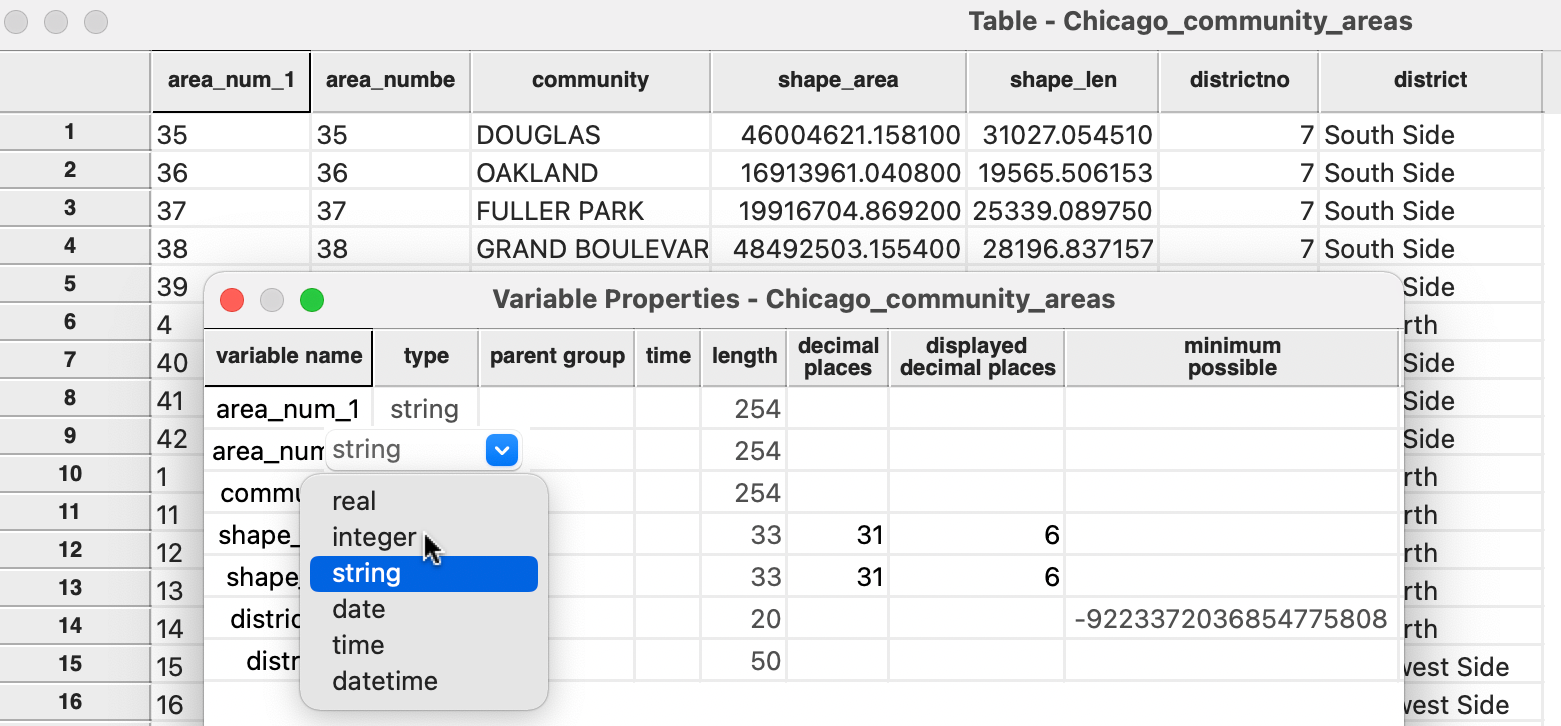
Figure 2.17: Edit variable properties
In the table, the area identifiers - both area_num_1 and area_numbe (which are identical) - are left-aligned in their columns. This indicates they are character variables and not in a numeric format.
By selecting the proper integer format from the drop down list, the change is immediate. As mentioned, the most common use of this functionality is to change string variables to a numeric format.
In order to make the change permanent, the table needs to be saved, either by selecting the middle icon in the toolbar in Figure 2.1, or by means of File > Save. Note that this will overwrite the current files. To avoid this behavior, select File > Save As and specify a new file name.
To facilitate data table operations like Merge, the community area identifier must be changed to integer.
2.4.1.2 Formatting date/time variables
One special case where the Edit Variable Properties option is extremely useful is when information on the date and time of an observation is included in the data table. Typically, this is contained in a string variable, which does not allow for any operations such as searching or sorting. Instead, a special date/time format must be used, which requires converting from string to this format.
For example, this is the case for the observations in the Chicago Carjackings points data set. The third column of the data table in Figure 2.18 shows the Date as a string variable. Specifically, the first entry is 12/11/2020 11:45:00 PM, which lists the month, day and year, separated by a forward slash (/), followed by the time in hours, minutes and seconds (separated by a colon) and AM or PM.
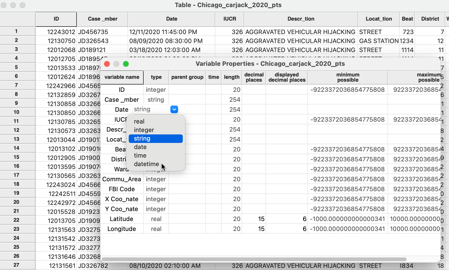
Figure 2.18: Create a date/time variable
Selecting datetime from the drop down list will change the format into a standard time expression, as in Figure 2.19. Note how the order of the information has changed to year-month-day and the time is in 24 hours, minutes and seconds (no more AM or PM). At this point, the date information can be manipulated by means of the Date/Time functions in the calculator (see Section 2.4.2.5).
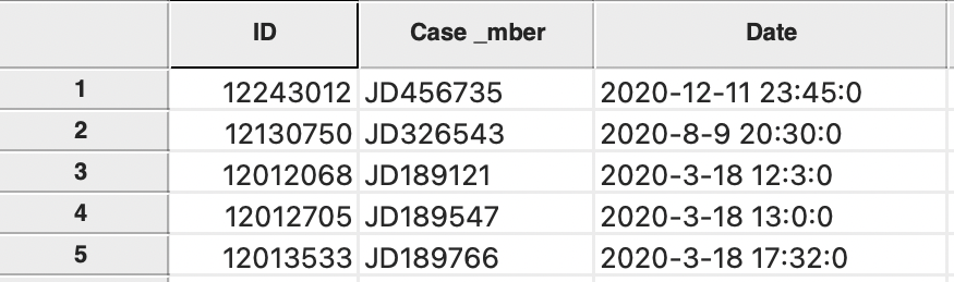
Figure 2.19: Date/time format
However, there is a catch. GeoDa recognizes many date-time formats, but not all. The default ones are listed under the Data tab of the GeoDa Preference Setup (see also Appendix A). Sometimes, the particular format used is not part of the default. It therefore may have to be added to the list, as shown in Figure 2.20. For example, the proper entry for the carjacking format is %m/%d/%Y %I:%M:%S %p, the last item in the Date/Time formats list. This follows the standard format for date and time information.6
Once a customized format is included into the setup interface, it will be recognized in all future instances of datetime format conversion.
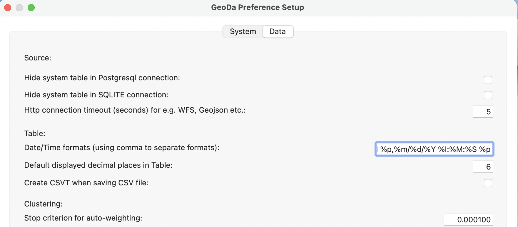
Figure 2.20: Customizing the date/time format
2.4.1.3 Other variable operations
The other variable operations listed in the drop down list in Figure 2.16 are mostly self-explanatory. For example, a new variable can be included through Add Variable (its value is obtained through the Calculator, see Section 2.4.2), or variables can be removed by means of Delete Variable(s). Rename Variable operates on a specific column, which needs to be selected first.
Two more obscure options are Encode and Setup Number Formatting. The default encoding in GeoDa is
Unicode (UTF-8), but a range of other encodings that support non-western characters are available as well.
The default numeric formatting is to use a period for decimals and to separate thousands by a comma, but the
reverse can be specified as well, which is common in Europe.
2.4.1.4 Operations on the table
The columns, rows and cells of the table can be manipulated directly, similar to spreadsheet operations. For example, the values in a column can be sorted in increasing or decreasing order by clicking on the variable name. A > or < sign appears next to the variable name to indicate the sorting order. The original order can be restored by sorting on the row numbers (the left-most column).
Individual cell values can be edited by selecting the cell and entering a new value. As is always the case in GeoDa, such changes are only permanent
after the table is saved.
Specific observations can be selected manually by clicking on their row number (selection through queries is covered in Section 2.5). The corresponding entries will be highlighted in yellow. Additional observations can be added to the selection in the usual way, for example, by means of shift-click (or another key combination, depending on the operating system). The selected observations can be located at the top of the table for easy reference by means of Move Selected to Top.
Finally, the arrangement of the columns in the table can be altered by dragging the variable name and moving it to a different position. This is often handy to locate related variables next to each other in the table for easy comparison when the original layout is not convenient.
2.4.2 Calculator
The Calculator functionality provides a rudimentary interface to create new variables, transform existing variables and carry out a number of algebraic operations. It is limited to one operation at a time, so it is not suitable for bulk programming.
The Calculator interface contains six tabs, dealing, respectively, with Special functions, Univariate and Bivariate operations, Spatial Lag, Rates and Date/Time operations. Spatial Lag and Rates are advanced functions that are discussed separately in Chapters 6 and 12.
The calculator interface is shown in Figure 2.21, illustrated for the Bivariate operations. Each tab at the top includes a series of functions, either creating a new variable (Special), operating on a single variable (Univariate), two variables (Bivariate), or values contained in a special Date/Time format. The specific functions are selected from the Operator drop down list.
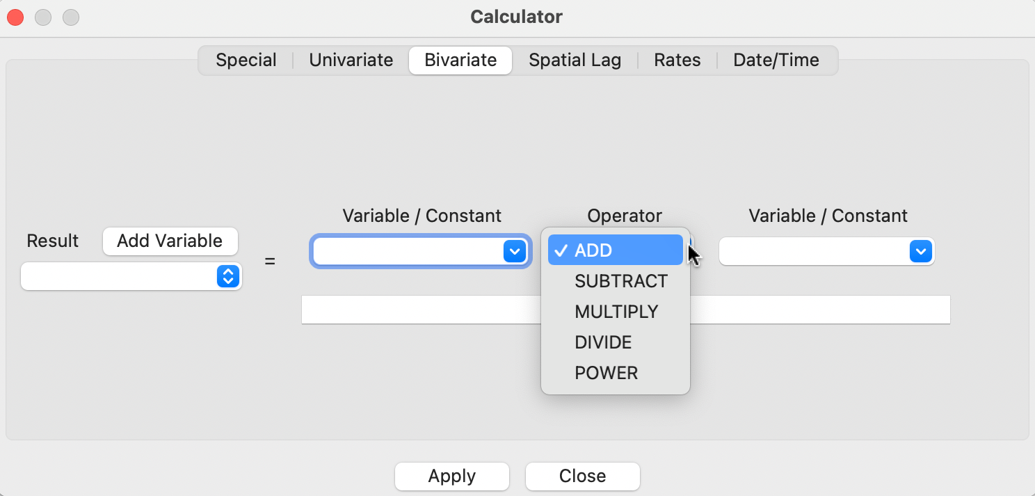
Figure 2.21: Calculator interface
Each operation begins by identifying a target variable in which the result of the operation will be stored. Typically, this will be a new variable, which is created by means of the Add Variable button located to the right of Result.7 This brings up an interface in which the Name for the new variable is specified, as well as its Type, its precision, and where to insert it into the table. The default is to place a new variable to the left of the first column in the table, but any other variable can be taken as a reference point (i.e., the new column is placed to the left of the specified variable). In addition, the new variable can also be placed at the right most end of the table (the last option in the list).
With the target variable specified, the actual calculations can be carried out by selecting the operation from the drop down list and choosing the variables involved. Again, to make the new variable permanent, the data table needs to be saved.
The various operations are briefly reviewed next.
2.4.2.1 Special functions
Special functions create a new variable, either a random variable, NORMAL or UNIFORM RANDOM, or the rank order of the current observations. The latter is generated by the ENUMERATE function. This yields a new variable with the current order of the observations. It is especially useful to retain the order of observations after sorting on a given variable, such as the rank order corresponding to a given statistic.
2.4.2.2 Univariate functions
Operations that pertain to a single variable are included in the Univariate drop down list. ASSIGN allows a variable to be set equal to any other variable, or to a constant (the typical use). The next five operations are straightforward transformations, including NEGATIVE (change the sign), INVERT, SQUARE ROOT, and base 10 and natural LOG.
SHUFFLE randomly permutes the values for a given variable to different observations. This is an efficient way to implement spatial randomness, i.e., an allocation of values to locations, but where the location itself does not matter (any location is equally likely to receive a given observation value).
2.4.2.3 Variable standardization
The univariate operations also include five types of variable standardization. The most commonly used is undoubtedly STANDARDIZED (Z). This converts the specified variable such that its mean is zero and variance one, i.e., it creates a z-value as \[z = \frac{(x - \bar{x})}{\sigma(x)},\] with \(\bar{x}\) as the mean of the original variable \(x\), and \(\sigma(x)\) as its standard deviation.
A subset of this standardization is DEVIATION FROM MEAN, which only computes the numerator of the z-transformation.
An alternative standardization is STANDARDIZED (MAD), which uses the mean absolute deviation (MAD) as the denominator in the standardization. This is preferred in some of the clustering literature, since it diminishes the effect of outliers on the standard deviation (see, for example, the illustration in Kaufman and Rousseeuw 2005, 8–9). The mean absolute deviation for a variable \(x\) is computed as: \[\mbox{mad} = (1/n) \sum_i |x_i - \bar{x}|,\]
i.e., the average of the absolute deviations between an observation and the mean for that variable. The estimate for \(\mbox{mad}\) takes the place of \(\sigma(x)\) in the denominator of the standardization expression.
Two additional transformations that are based on the range of the observations, i.e., the difference between the maximum and minimum. These the RANGE ADJUST and the RANGE STANDARDIZE options.
RANGE ADJUST divides each value by the range of observations: \[r_a = \frac{x_i}{x_{max} - x_{min}}.\] While RANGE ADJUST simply re-scales observations in function of their range, RANGE STANDARDIZE turns them into a value between zero (for the minimum) and one (for the maximum): \[r_s = \frac{x_i - x_{min}}{x_{max} - x_{min}}.\]
Note that any standardization is limited to one variable at a time, which admittedly is not very efficient. However, most analyses where variable standardization is recommended, such as in the multivariate clustering techniques covered in Volume 2, include a transformation option that can be applied to all the variables in the analysis simultaneously. The same five options as discussed here are available to each analysis.
2.4.2.4 Bivariate operations
The bivariate functionality includes all classic algebraic operations. The target variable is selected from the drop down list on the left in Figure 2.21. Then the respective variables (or a constant) are entered in the dialog with the appropriate operation selected from the list. This includes ADD, SUBTRACT, MULTIPLY, DIVIDE and POWER.
2.4.2.5 Date and time functions
The calculator also contains limited functionality to operate on date and time fields. In practice, this can be quite challenging, due to the proliferation of formats used to define variables that pertain to dates and time, as encountered in Section 2.4.1.2.
The Date/Time operators implement functions to extract specific parts from the data format and store them as integer variables. These include Get Year, Get Month, Get Day, Get Hour, Get Minute and Get Second. The resulting integer variable can then be used to carry out queries (see Section 2.5.1).
2.4.3 Merging tables
An important operation on tables is the ability to Merge new variables into an existing data set, or, in other words, to join an external table to the currently active one.
For example, the Chicago_community_areas.shp file only contains information on the community area boundaries, but no actual data. On the other hand, the Chicago_CCA_profiles_2020.csv file contains a wealth of socio-economic data, but no spatial information other than the ID number for the community area. In order to combine the spatial information with the non-spatial data, the two tables need to be joined.
With the community area boundaries loaded, the Table > Merge option brings up the dialog shown in Figure 2.22.
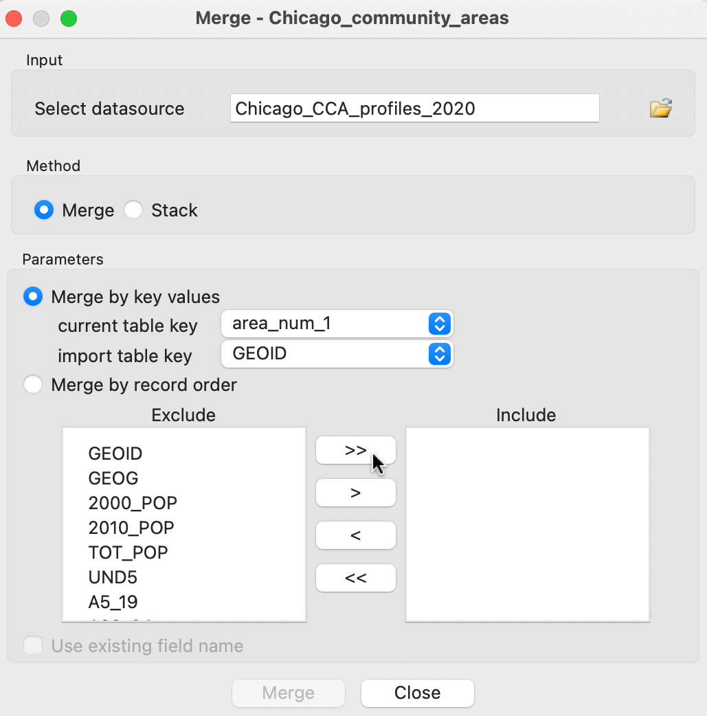
Figure 2.22: Merge dialog
The first step is to load the file to be merged (Select datasource). In Figure 2.22 this is Chicago_CCA_profiles_2020.csv. The default method is Merge, but Stack is supported as well. The latter operation is used to add observations to an existing data set.
Rather than relying on the order of the observations in both data sets, it is best practice to carry out a merging operation by selecting a key. This is a variable that contains (numeric) values that match the observations in both data sets. Using a key is superior to merging by record order, since there is often no guarantee that the actual ordering of the data in the two sets is the same, even though it may seem so in the interface (such as the table view). In the example, area_num_1 is the key in the first data set (assuming it has been reformatted to integer) and GEOID the key in the second.
The variables to be merged are selected by moving their names from the Exclude box to the Include box. Using the >> button selects all of them.
Upon clicking the Merge button at the bottom of the dialog, the new variables will be added to the current data table, unless there is a potential conflict of variable names. This conflict can be two-fold. First, when variables have identical names in both data sets, they need to be differentiated. If that is the case, alternatives are suggested in a dialog. These alternatives are not always the most intuitive and can be readily edited in the entry box. One exception to this is when you do not want to merge in the duplicate fields. Checking the box Use existing field name makes sure that only the original columns are kept.
A second potential conflict is when the variable name to be included contains more than 10 characters. In csv input files, there are no constraints on variable name length, but the dbf format used for the attribute values in a shape file format has a limit of 10 characters for a variable name. Again, an alternative will be suggested in the dialog, but it can be easily edited (as long as it stays within the 10 character limit).8
The merged tables are shown in Figure 2.23. By keeping the identifiers for both data sets in the merged table (respectively area_num_1 - in the first column - and GEOID - in the 8th column), one can easily verify that the observations are lined up correctly.
As before, the merger only becomes permanent after a File > Save operation.
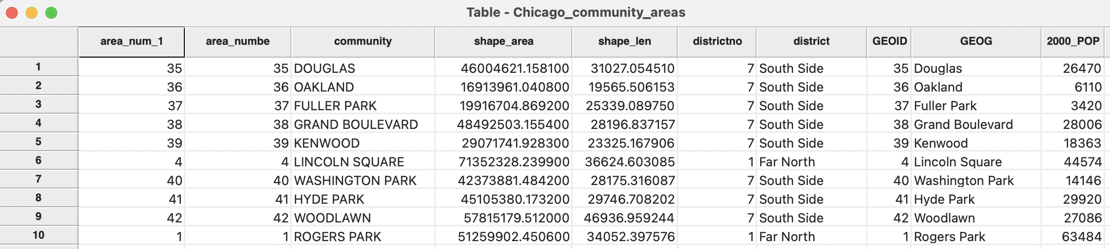
Figure 2.23: Merged tables
Note that the merge operation in GeoDa implements a left join, in the sense that only observations that match the ID in the current table are included in the merged table. Specifically, if the table to be merged does not contain certain observations, the corresponding entries in the merged table will be missing values. Also, if the table to be merged contains observations that are not part of the current table, they will be ignored. Other forms of joins are not currently implemented.
Specifically, %m stands for two digit month (including a leading zero), %d for two digit day (again, including a leading zero), %Y for the year in full four digits, %I for the hour in 12 hour segments (this requires AM or PM in addition), %M for minutes in two digits, %S for seconds in two digits and %p for AM or PM.↩︎
A new variable can also be created directly from the table options menu as Table > Add Variable.↩︎
The same problem can occur when using File > Save As to convert a csv file to the dBase format. Here too, a dialog will suggest alternative variable names, which can be edited.↩︎