13.3 Positive and negative spatial autocorrelation
Rejecting the null hypothesis of spatial randomness suggests that there is some spatial structure in the data. When the focus in on dependence (as opposed to heterogeneity), the two alternative hypotheses are positive and negative spatial autocorrelation. Unlike what holds for the familiar notion of correlation (without space), negative spatial autocorrelation is not simply the negative of positive spatial autocorrelation, i.e., a negatively sloped linear relation contrasted with a positively sloped on. Negative spatial autocorrelation yields a totally different type of spatial pattern.
13.3.1 Positive spatial autocorrelation
Positive spatial autocorrelation implies that like values in neighboring locations occur more frequently than they would under spatial randomness. This results in an impression of clustering, the clumping in space of like values. These like values can be either high (hot spots) or low (cold spots). The key aspect is attribute similarity among neighboring locations.
Figure 13.5 illustrates strong positive spatial autocorrelation on a 10 \(\times\) 10 regular grid.97 While the pattern may suggest some clustering, this is very difficult to assess by eye, especially relative to the true spatially random pattern of Figure 13.2.
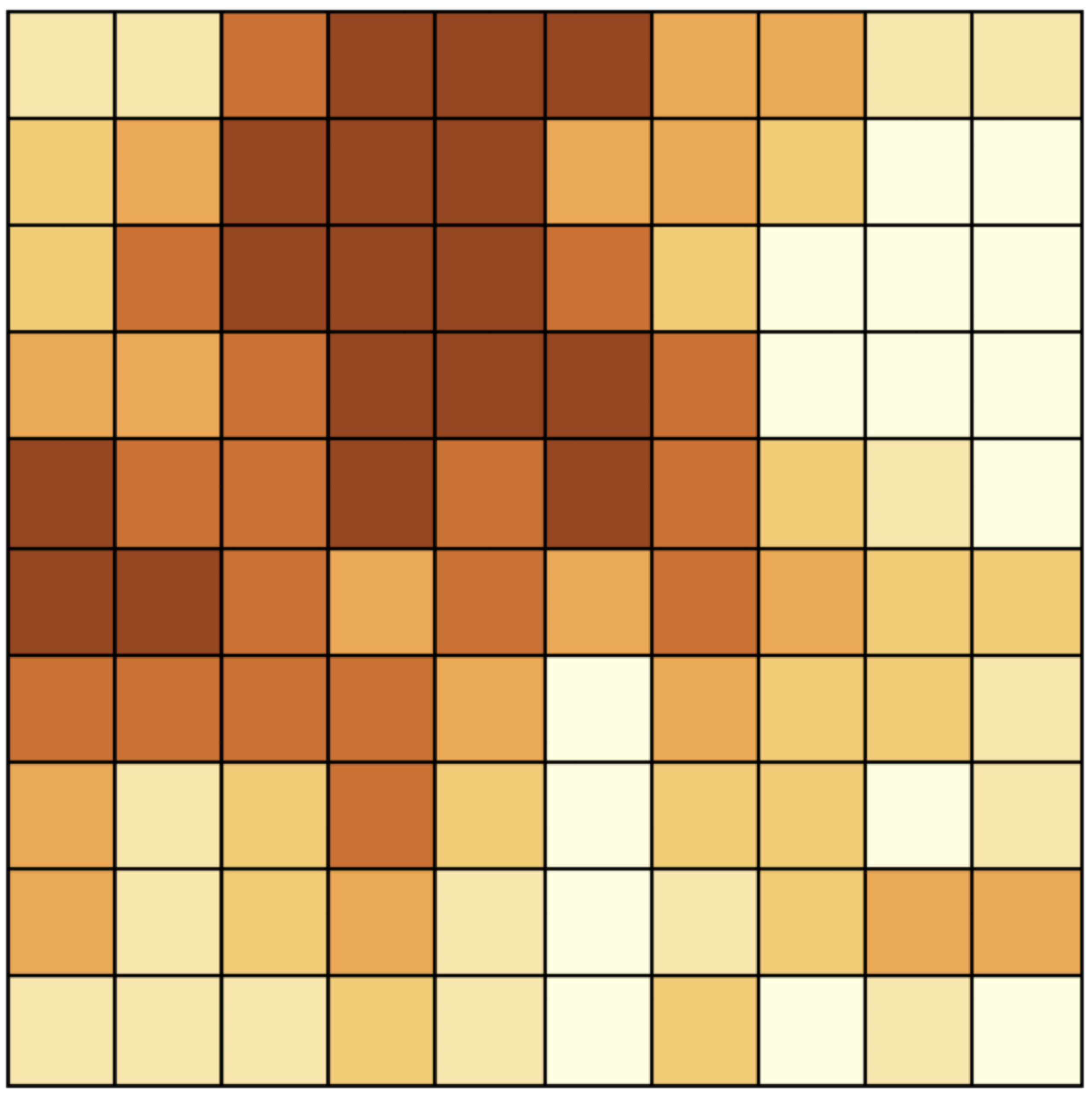
Figure 13.5: Positive spatial autocorrelation
13.3.2 Negative spatial autocorrelation
Negative spatial autocorrelation is suggested when neighboring values are more dissimilar than they would be under spatial randomness. This typically yields a checkerboard-like pattern. The dissimilarity is often associated with spatial heterogeneity, although the latter is not limited to neighboring units. Negative spatial autocorrelation implies alternating high and low values, whereas spatial heterogeneity can pertain to larger regions that include many neighbors.
Figure 13.6 illustrates how difficult it is to distinguish negative spatial autocorrelation from spatial randomness (Figure 13.2). It portrays a strong degree of negative spatial autocorrelation on a 10 \(\times\) 10 regular grid.98 Whereas there are quite a few dark values surrounded by lighter ones, this is by no means a perfect checkerboard.
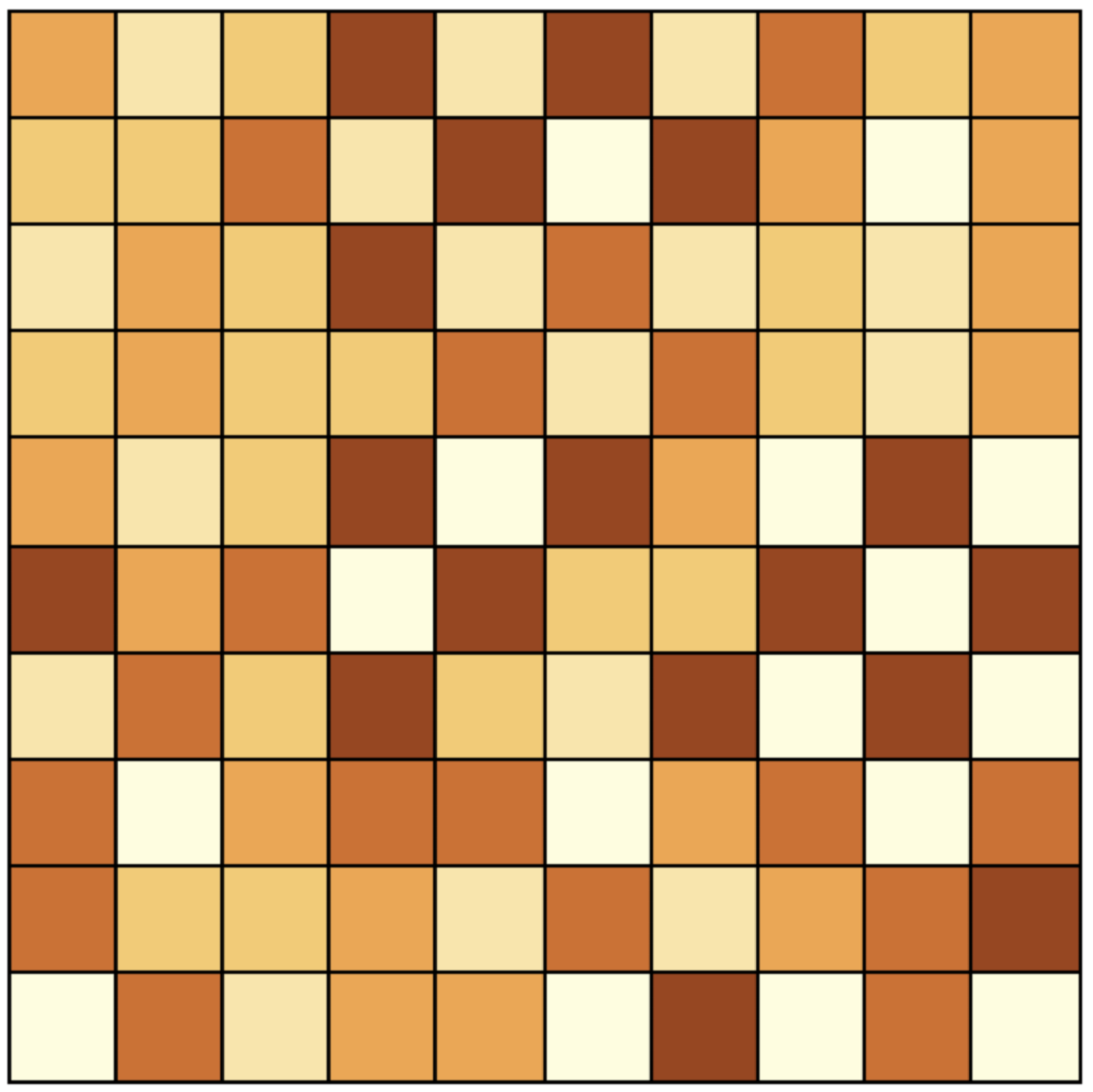
Figure 13.6: Negative spatial autocorrelation