18.5 Local Neighbor Match Test
An alternative approach to visualize and quantify the trade off between geographical and attribute similarity was suggested by Anselin and Li (2020) in the form of what is called a Local Neighbor Match Test. The basic idea is to assess the extent of overlap between k-nearest neighbors in geographical space and k-nearest neighbors in multi-attribute space.
In GeoDa, this becomes a simple intersection operation between two k-nearest neighbor weights matrices (see Section 11.6.1). One matrix is derived from the distances in multi-attribute space, the other using geographical distance. With the intersection in hand,
the probability that an overlap occurs between the two neighbor sets can be quantified. This corresponds to the probability
of drawing \(v\) common neighbors from the \(k\) out of \(n - 1 - k\) possible choices as neighbors,
a straightforward combinatorial calculation.
More formally, the probability of \(v\) shared neighbors out of \(k\) is:
\[p = C(k,v).C(N-k,k-v) / C(N,k),\]
where \(N = n - 1\) (one less than the number of observations), \(k\) is the number of nearest neighbors considered
in the connectivity graphs, \(v\) is the number of neighbors in common, and \(C\) is the combinatorial operator.
Alternatively, a pseudo p-value can be computed based on a permutation approach, although that is not
pursued in GeoDa.
The degree of overlap can be visualized by means of a cardinality map, a special case of a unique values map. In this map, each location indicates how many neighbors the two weights matrices have in common. In addition, different p-value cut-offs can be employed to select the significant locations, i.e., where the probability of a given number of common neighbors falls below the chosen p.
In practice, the value of \(k\) may need to be adjusted (increased) in order to find meaningful results. In addition, the k-nearest neighbor calculation becomes increasingly difficult to implement in very high attribute dimensions, due to the empty space problem (Section 8.2.1).
The idea of matching neighbors can be extended to distances among variables obtained from dimension reduction techniques, such as multidimensional scaling, covered in Volume 2 (see also the more detailed discussion in Anselin and Li 2020).
In contrast to the approach taken for the Multivariate Local Geary, the local neighbor match test focuses on the pairwise distances directly, instead of converting these into a weighted average. Both measures have in common that they focus on squared distances in attribute space, rather than a cross-product as in the Moran statistics.
18.5.1 Implementation
The Nearest Neighbor Match test is invoked as the last item in the drop down list associated with the Cluster Maps toolbar icon, or, from the menu, as Space > Local Neighbor Match Test. This is followed by a dialog to select the variables.
In addition to the variable names, the dialog includes options for four important parameters. The Number of Neighbors specifies the range for which the match is explored, i.e., the value of \(k\) in the k-nearest neighbor weights that are computed under the hood. In the example, 6 is used, to allow comparison with the other approaches considered in this chapter. Next is the Variable Distance Function, with Euclidean as the default, but Manhattan distance as the other option. A third option pertains to the Geographic Distance Metric. Here again, Euclidean Distance is the default, but Arc Distance is available as well, for the case where the map layer is unprojected. Finally, Transformation offers six options to adjust the variables: Raw, Demean, Standardize (Z), Standardize (MAD), Range Adjust, and Range Standardize. The default of Standardize (Z) is the recommended approach. With this information, the two k-nearest neighbor weights are constructed and the cardinality of the intersection computed.
In the illustration, the same three variables are employed as for the Multivariate Local Geary. Before moving to the actual test, the logic of the approach is detailed.
18.5.1.1 Intersection between connectivity graphs
Figure 18.12 shows the connectivity graphs corresponding to geographic 6 nearest neighbors and the multi-attribute 6 nearest neighbors (see Section 11.4.4). The graph on the left takes on a familiar form, but the graph on the right suggests that a lot of multivariate connections span large geographic distances.
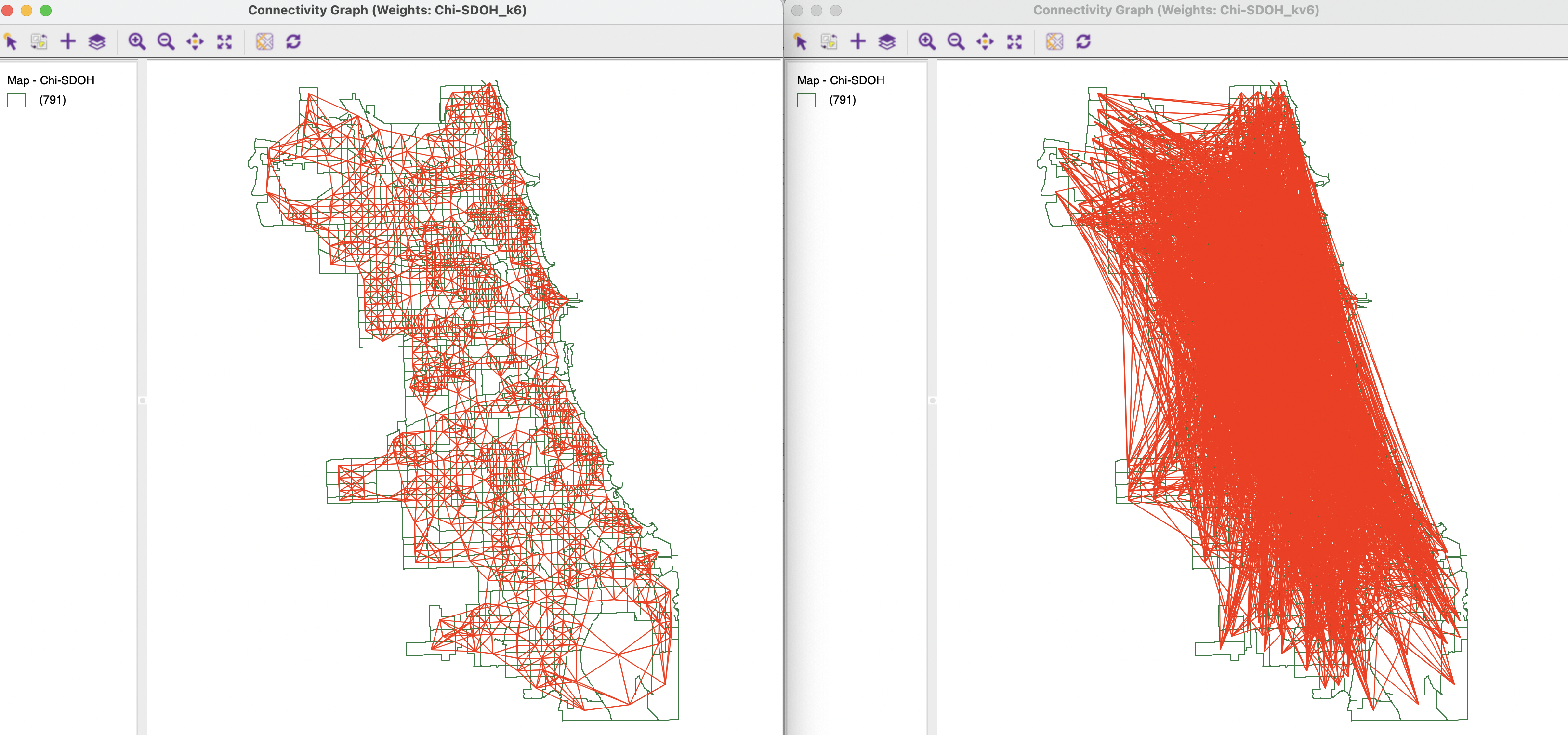
Figure 18.12: K nearest neighbor connectivity graphs
The intersection between the two weights yields the connectivity graph illustrated in Figure 18.13.122 The result is very sparse, with most intersections consisting of a single link. This graph structure forms the point of departure for the Local Neighbor Match Test.
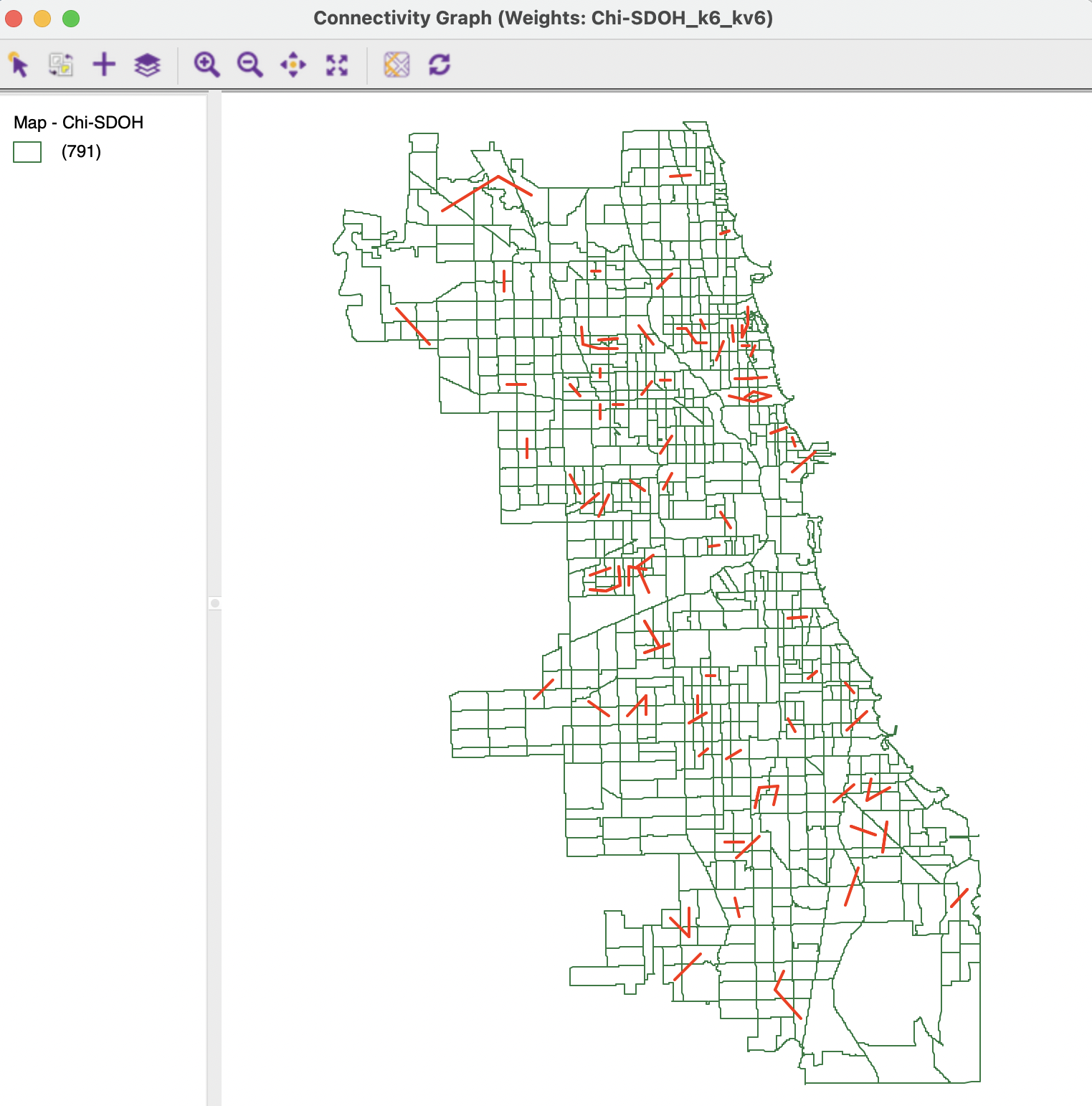
Figure 18.13: Intersection of K nearest neighbor connectivity graphs
18.5.1.2 Testing the local neighbor match
The degree of local neighbor match is visualized by means of a cardinality map, as shown in Figure 18.14. This is a special case of a unique values map, where the categories correspond to the number of matching neighbors. In this example, there are 101 observations with a single match, and 10 observations with two matches.
The map is accompanied with a prompt to save the cardinality (default variable card) and the associated probability (default variable cpval). Note that no probabilities are computed for the cases where no matches occur.
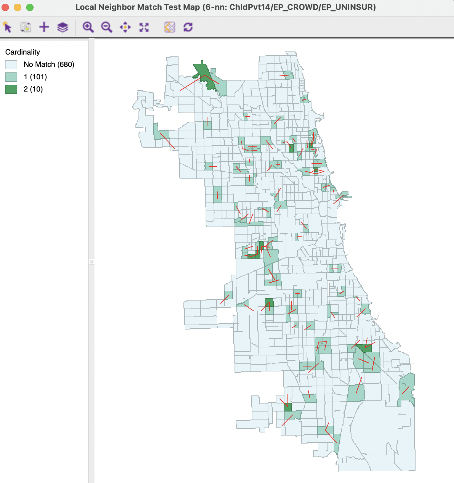
Figure 18.14: Local neighbor match cardinality map
Even though the largest number of matches is only two, such an occurrence is very rare under spatial randomness, corresponding with a p-value of 0.0007. The 10 such identified observations are highlighted in Figure 18.15, with the matching links shown in red.
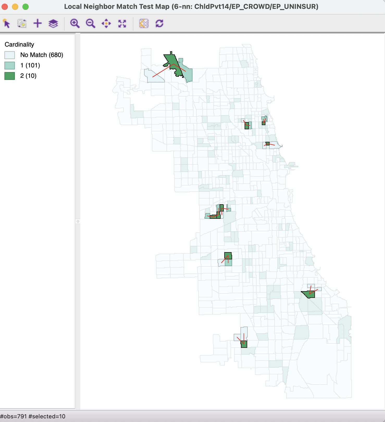
Figure 18.15: Local neighbor match significance map
Figure 18.16 provides a better sense of the rarity of the coincidence between geographic and multi-attribute nearest neighbors. The two sets of neighbors are shown for the 10 highlighted locations. It is clear that several nearest neighbors in attribute space are not so close in geographic space, confirming the tension between the two notions of similarity.
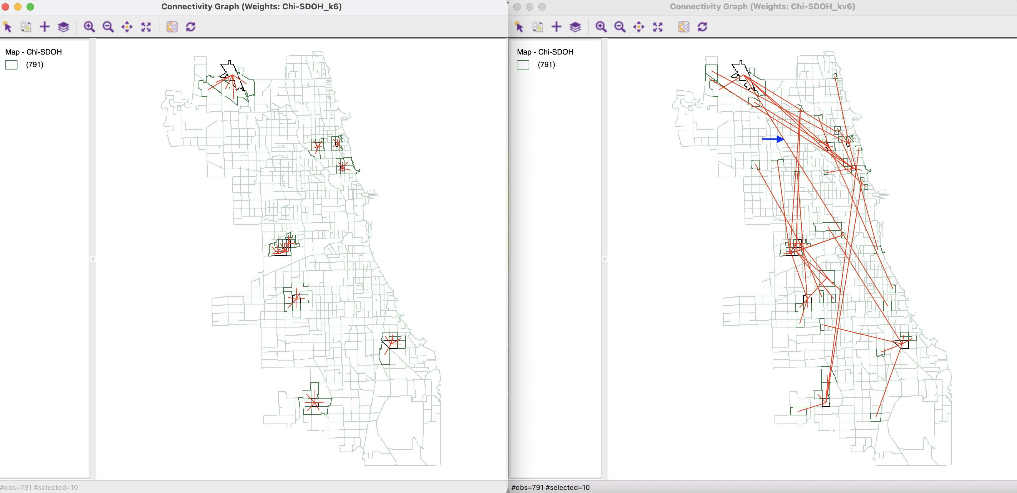
Figure 18.16: Local neighbor significant matches
18.5.2 Local neighbor match and Multivariate Local Geary
A final perspective on what insights the local neighbor match provides follows from a comparison with the interesting locations identified by means of the Multivariate Local Geary. In Figure 18.17, the 10 locations in the Local Neighbor Match Test map on the left are linked to their corresponding observations in the Multivariate Local Geary cluster map on the right. Of the 10, six are also identified by the Multivariate Local Geary, but four are not. Those four are instances where the average distances in attribute space to the geographic neighbors are much larger than the individual distances for the nearest neighbors in attribute space (as opposed to all the neighbors).
This can be assessed by investigating the linkage structure for the affected observations in the right hand panel of Figure 18.16. For example, for the census tract identified by the green rectangle in Figure 18.17, several of the nearest attribute neighbors are far away in geographic space, as illustrated by the link highlighted by the blue arrow in Figure 18.16, as well as its other links beyond the first two neighbors.
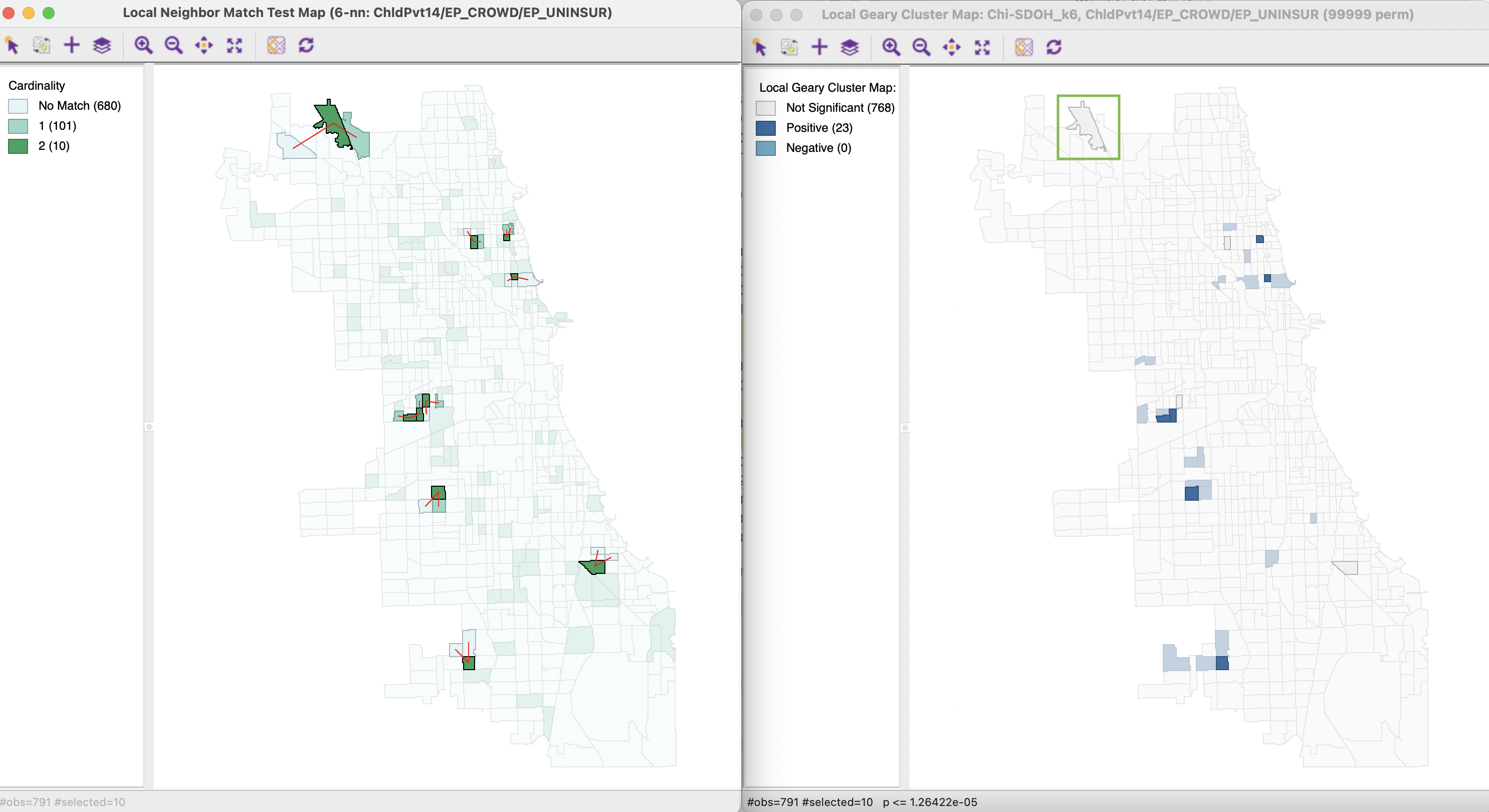
Figure 18.17: Local neighbor match and Multivariate Local Geary
By focusing on a different aspect of the locational-attribute similarity trade-off, the Local Neighbor Match Test provides yet another avenue to explore multivariate local clusters. However, as pointed out, this approach does not scale well to a large number of variables, since the empty space problem creates a large computational burden for the calculation of k-nearest neighbors in high-dimensional attribute space.
This is accomplished by means of the Intersection command in the Weights Manager.↩︎