6.2 Choropleth Maps for Rates

The distinguishing characteristic of the implementation of maps for rates or proportions in GeoDa is the explicit computation of the ratio by specifying variables for the numerator and the denominator. The map types are the same as those reviewed in Chapters 4 and 5. In addition, there are some options to save the rates in the table.

Before delving into the specifics, I first discuss the important difference between spatially extensive and spatially intensive variables. Only the latter should be used in a choropleth map. Next, I outline the implementation of the rate maps and some important options.

6.2.1 Spatially extensive and spatially intensive variables

Many variables in empirical studies are directly correlated with the size of the observational unit. Examples include total population, number of housing units, count of crimes, etc. In essence, everything else being the same, larger observational units should have larger values for such variables. They are therefore referred to as spatially extensive, being directly related to the size of the observational unit. Unless all spatial units have the same area, this can lead to spurious suggestions of importance or outlier values. Consequently, choropleth maps, which use the area of the spatial unit to represent observations, are not an appropriate application for spatially extensive variables.

Instead, the variables should be standardized in some fashion, so that they reflect intrinsic variation, rather than variation in the size of the observational unit. This is readily accomplished by dividing by some measure of size. The classic example is to use the population at risk, such as the population exposed to the risk of a disease. This implies that the rate is interpreted as an estimate for the underlying risk (see Section 6.4.1). Alternatives are total area (resulting in density measures), or some other total, such as total population (resulting in per capita measures), without the implication of measuring an underlying risk. The resulting spatially intensive variables are appropriate for thematic mapping.

More formally, if \(O_i\) is the value for the numerator in area \(i\), and \(P_i\) is the corresponding denominator, then the raw or crude rate or proportion follows as: \[r_i = \frac{O_i}{P_i}.\]

To illustrate this concept, consider the box maps in Figures 6.1 and 6.2, depicting, respectively, population (pop) and population density (popdens), and GDP (gdp) and GDP per capita (gdpcap) for the municipios in the state of Ceará. The left panel pertains to the spatially extensive variable, while the right-hand panel shows the corresponding spatially intensive variable.

Whereas the population box maps suggests 10 outliers, several of which are spread throughout the state, the population density map has 13 outliers, mostly concentrated around the urban area of Fortaleza. Also, as highlighted in the two maps, several of the larger areas that rank in the upper quartile for total population, drop to the first quartile in terms of population density, i.e., after the area of the municipios is corrected for (their colors changes from browns to blues). In addition, most of the outliers in the larger (rural) areas, are no longer characterized as such in the population density map.

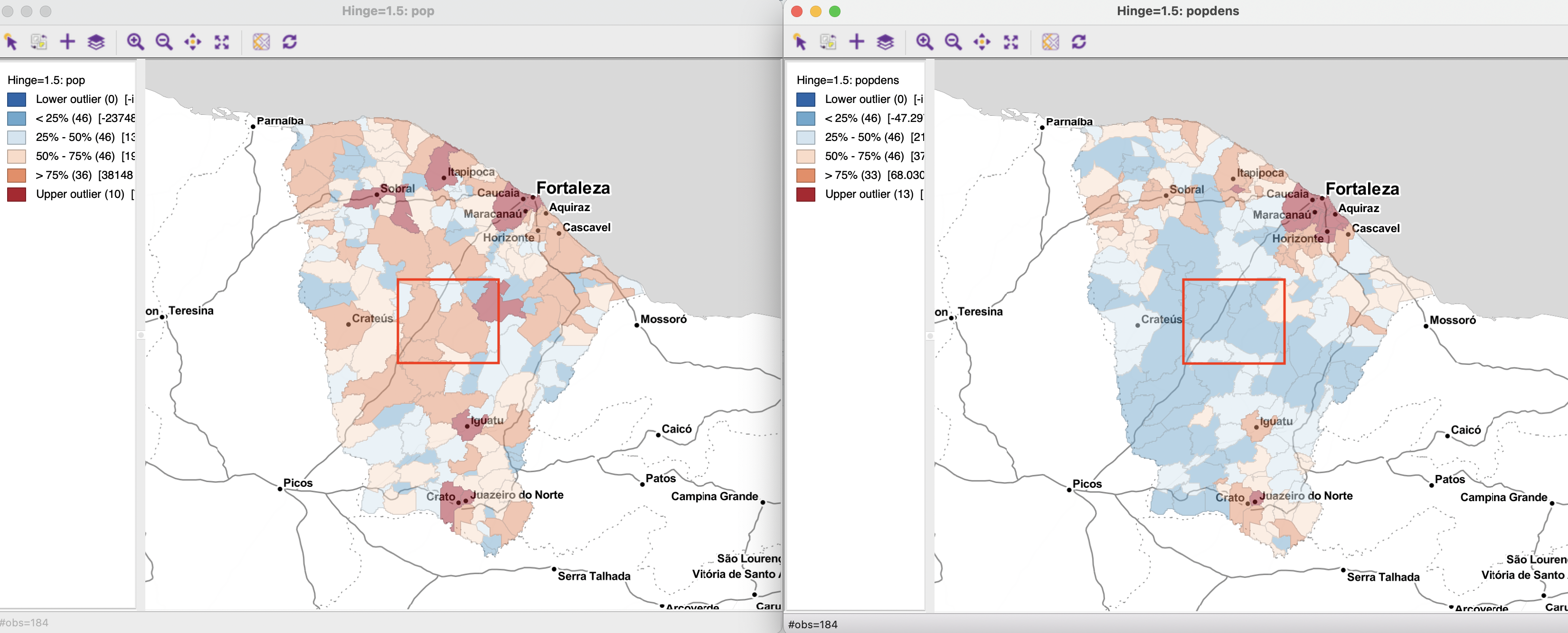
Figure 6.1: Population and population density

A similar phenomenon occurs in the maps for total GDP and GDP per capita. The number of outliers for GDP (a highly skewed variable) drops from 25 to 18 in the per capita map. Again, most of the larger (and rural) areas drop in the ranking, highlighted by their change in color from browns to blues.

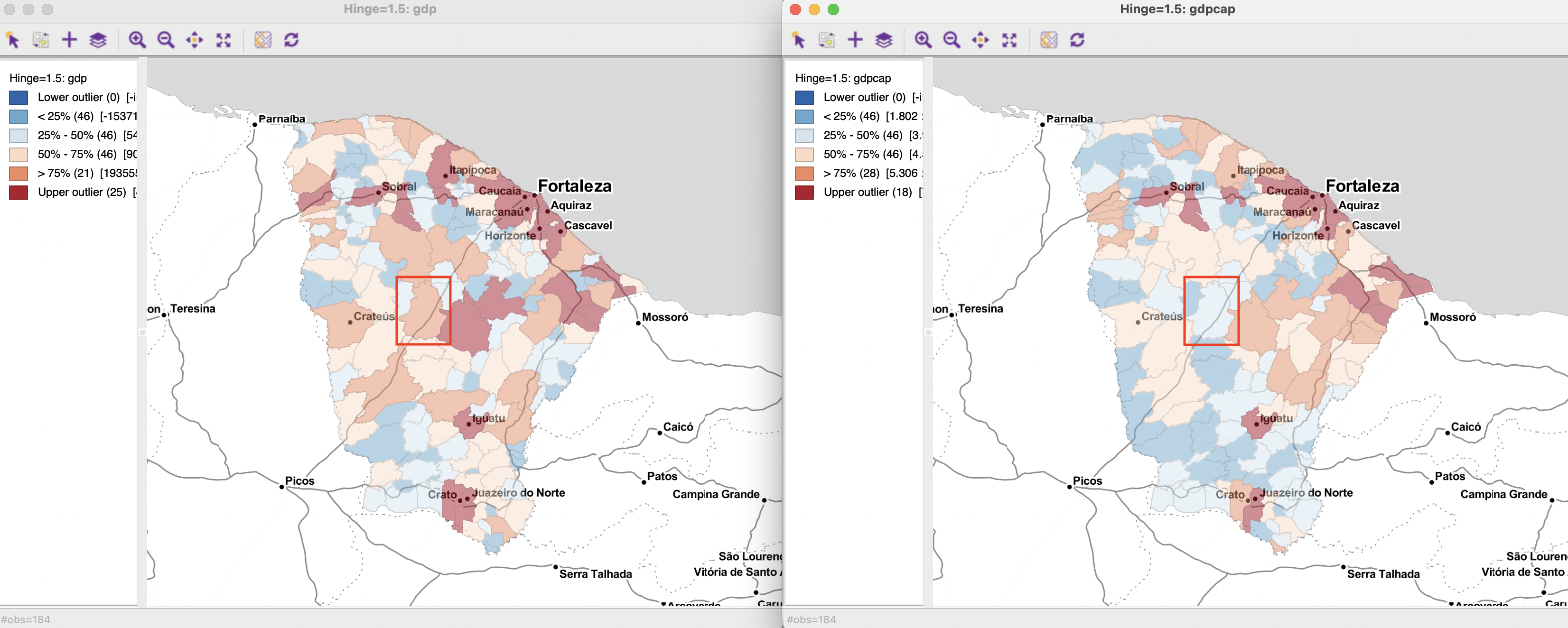
Figure 6.2: GDP and GDP per capita

In sum, a proper indication of the variability in the spatial distribution of the variable of interest is only obtained when the latter is converted to a spatially intensive form.

6.2.2 Raw rate map

A Raw Rate or crude rate map is invoked from the map menu or toolbar icon in the usual fashion, by selecting the bottom item in the interface from Figure 4.2: Map > Rates-Calculated Maps > Raw Rate. Alternatively, it can be created from an existing map window by selecting Rates in the list of map options (Figure 4.8).

In contrast to the previous maps, there is not a query for a single variable, but instead both the numerator (Event Variable) and denominator (Base Variable) of the ratio need to be specified, as shown in Figure 6.3. In the example, the respective variables are gdp and pop. The drop down list provides all the available map types. Here, a Box Map with hinge 1.5 is selected, resulting in the map shown in Figure 6.4.

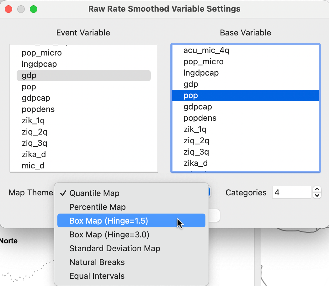
Figure 6.3: Rate map interface

Everything is the same as before, except that the map heading spells out both the numerator and denominator variables: Raw Rate gdp over pop. Specifically, the map is identical to the right-hand panel in Figure 6.2, which uses the gdpcap variable from the data table, rather than computing the ratio explicitly.

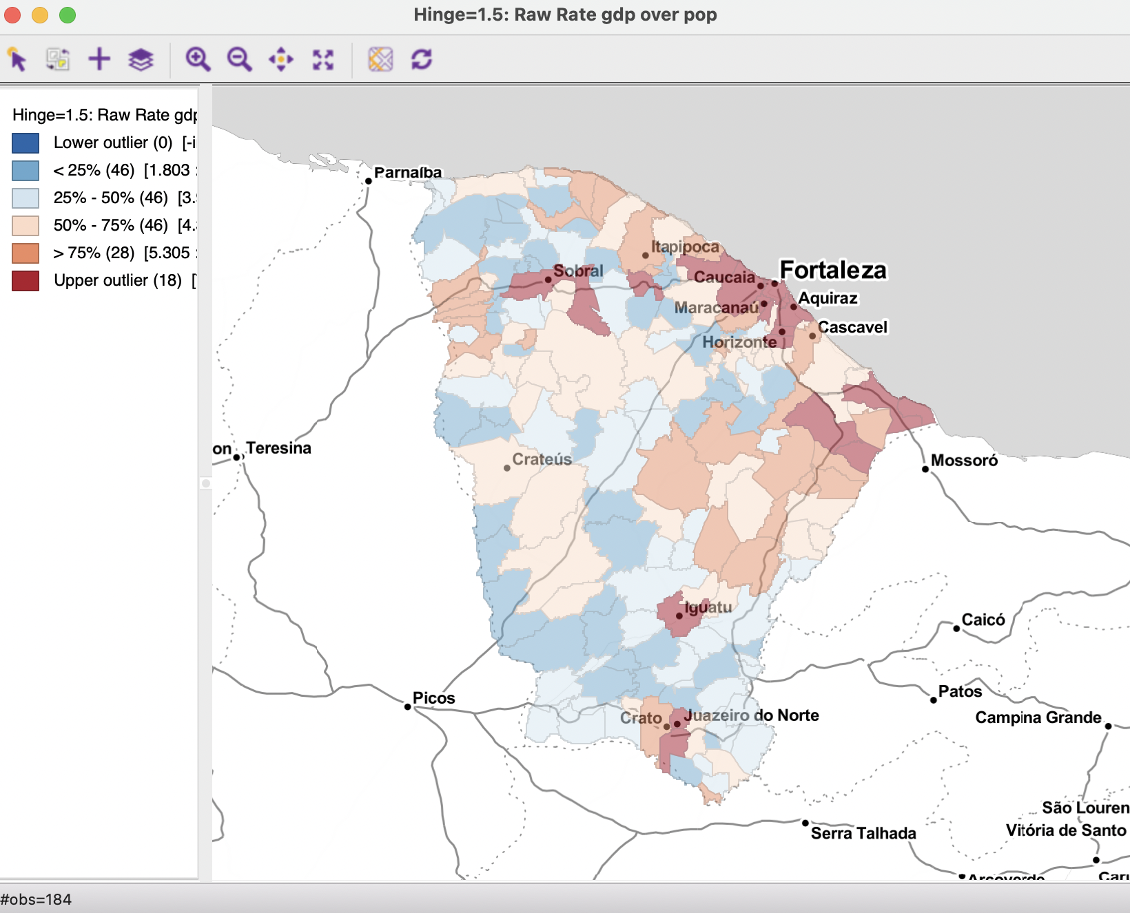
Figure 6.4: GDP per capita as a rate map

A rate map retains all the standard options of a map in GeoDa (see Section 4.5). Two additional features are Rates and Save Rates. Rates brings up a list of the different rate map options, since these are not available in the Change Current Map Type function in the main options menu. The Save Rates option allows for the calculated rates to be added to the data table. The default variable name for a raw rate is R_RAW_RT). As before, the new variable only becomes a permanent addition after a Save or Save As operation.

6.2.2.1 Rates in the table

Rates can also be computed directly in the table as part of the Calculator functionality, by selecting the Rates tab in the interface, shown in Figure 6.5 (see also Section 2.4.2 in Chapter 2). The particular type of rate is selected from the Method drop down list. In this example, the Raw Rate is used. As usual, a new variable must be added (here, r_gdpcap) and both the Event Variable (gdp) and Base Variable (pop) must be spelled out.

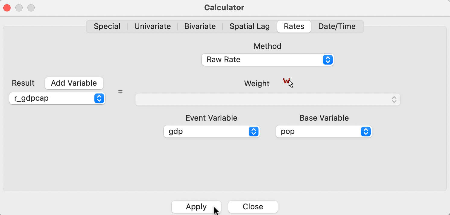
Figure 6.5: Rate calculation in table

Figure 6.6 illustrates the result. It shows side by side the original per capita GDP variable (gdpcap), the rate saved from the map window (R_RAW_RT), and the rate computed in the table (r_gdpcap). Rounded to the third decimal of precision, the values are identical.

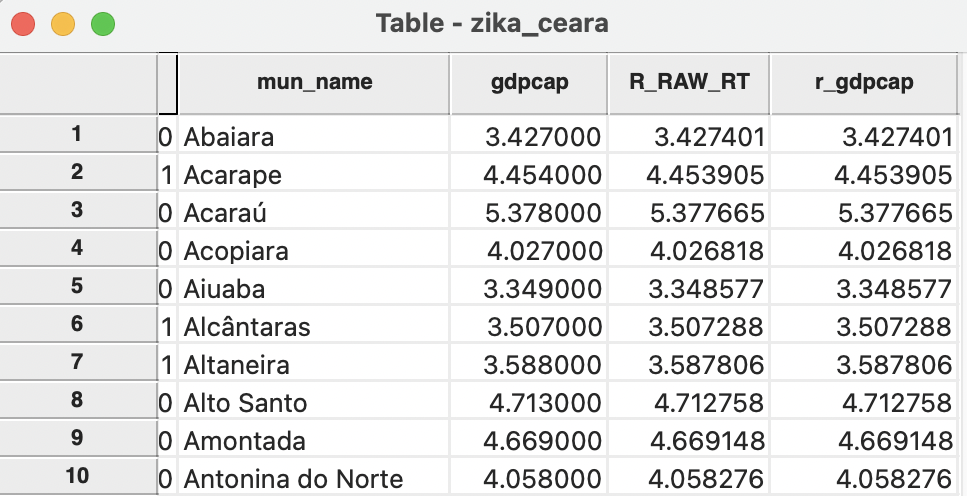
Figure 6.6: GDP per capita in table