3.4 Visualizing MDS

In addition to being integrated in a linking and brushing operation, as suggested in the previous discussion, the results of a MDS analysis can be visualized in a number of different ways. The main insight provided by the MDS scatter plot is the identification of observations that are close in multi-attribute space, summarizing the information contained in multiple variables down to two (or three) dimensions.

Two particularly insightful non-spatial visualizations can be considered. First, closeness in multi-attribute space can be highlighted by connecting a MDS scatter plot with a parallel coordinate plot. Also, a categorical variable can be introduced into the scatter plot, in a manner similar to the bubble chart discussed in Chapter 8 of Volume 1. For the sake of completeness, the 3D MDS scatter plot is briefly illustrated as well.

3.4.1 MDS and Parallel Coordinate Plot

Figure 3.11 highlights the PCP trajectory over the ten variables used in the analysis for two observations identified as close in the MDS scatter plot. The latter, shown in the right-hand panel, is the result of SMACOF for Manhattan distance, the same as Figure 3.9. The trajectories are very close and obtain (near) identical values for five out of the ten variables, with somewhat larger discrepancies for the others. The close pattern illustrates how the two-dimensional graph summarizes a pattern observed in high-dimensional attribute space.

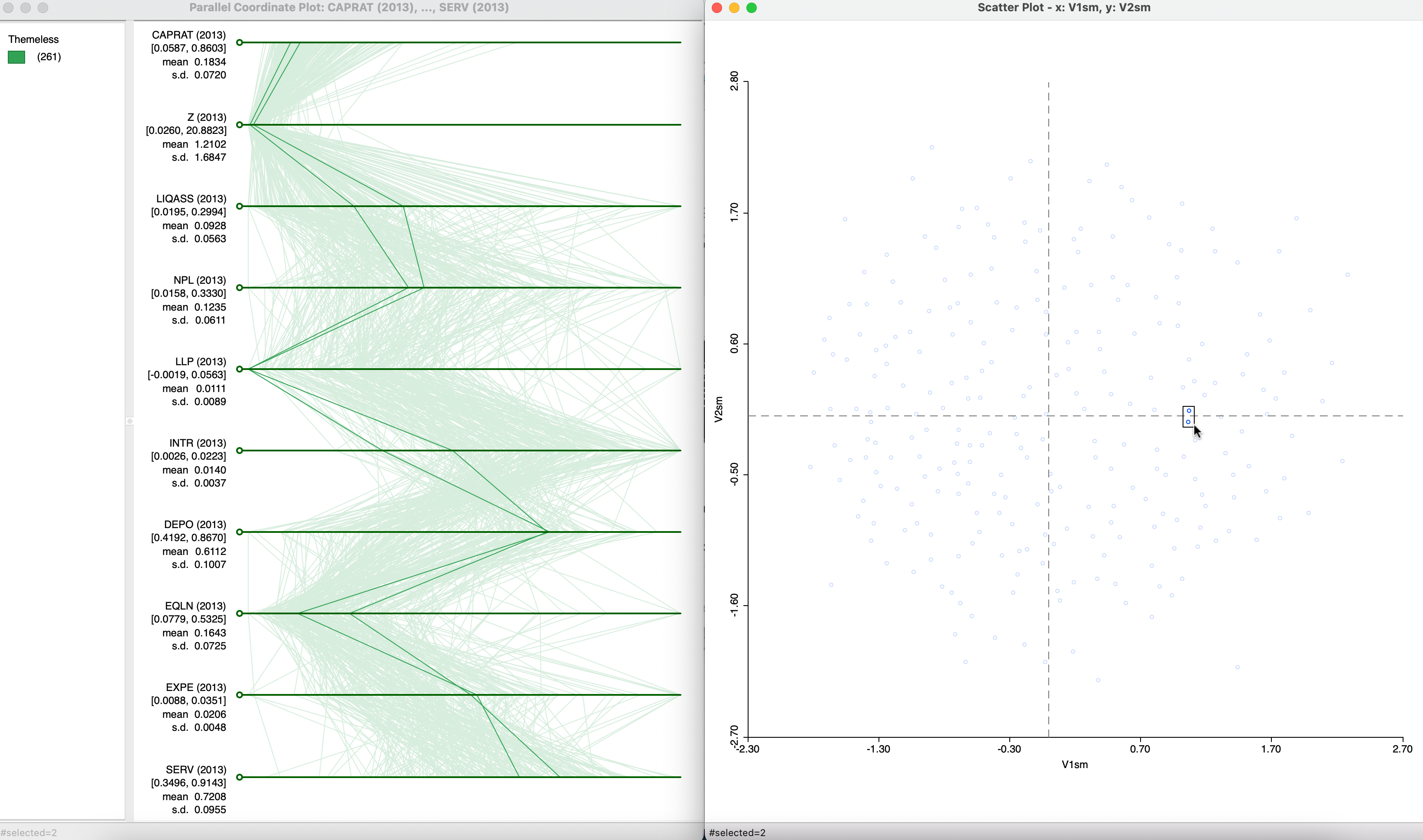
Figure 3.11: MDS and Parallel Coordinate Plot

3.4.2 MDS Scatter Plot with Categories

The MDS Settings dialog in Figure 3.2 contains a Category Variable option. With this option checked and an integer (category) variable selected, the MDS scatter plot turns into a type of bubble chart, with the scatter plot points taking on the color of the category to which they belong. This provides a way to assess whether observations that belong to the same category are also close in multi-attribute space, as summarized by their locations in the MDS scatter plot. In Figure 3.12, the category variable selected is REGCODE, the code for the region in which a community bank is located.

The plot on the right shows the points selected for the region of Trentino-Alto Adige (South Tirol), also highlighted in the map on the left. While some of the observations are close together, others are spread out over the scatter plot (again, a SMACOF MDS using Manhattan distance).

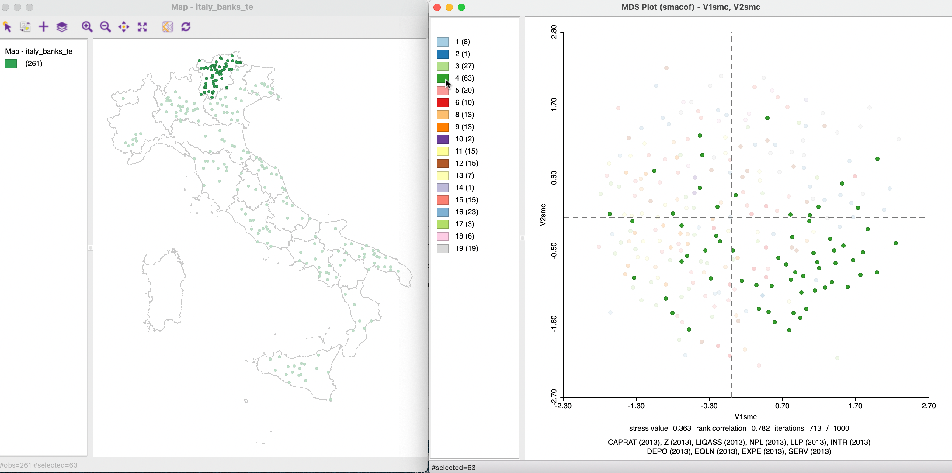
Figure 3.12: MDS with a Categorical Variable

Different categorical variables can be considered in this manner (both spatial as well as non-spatial) to assess the extent to which the categories correspond to groupings in multi-attribute space.

3.4.3 3-D MDS

The default setting for MDS analysis is to create a two-dimensional scatter plot. However, the option also exists to obtain results for three dimensions, by specifying 3 for the # of Dimensions option. The outcome for classic metric scaling is shown in Figure 3.13, side by side with the two-dimensional scatter plot (same as Figure 3.3). The variables under consideration are listed at the bottom of the graph, together with the stress value (0.295) and the rank correlation (0.866). Both measures of fit are better than in the two-dimensional case, which is not surprising, since less of a dimension reduction is involved.

At first sight, it would seem that the four close observations selected in the two-dimensional plot are also close in the 3D scatter plot. However, the perspective used to visualize the three-dimensional volume onto a flat surface can be misleading and the closeness can only be assessed after further manipulation, such as rotation and zooming in.

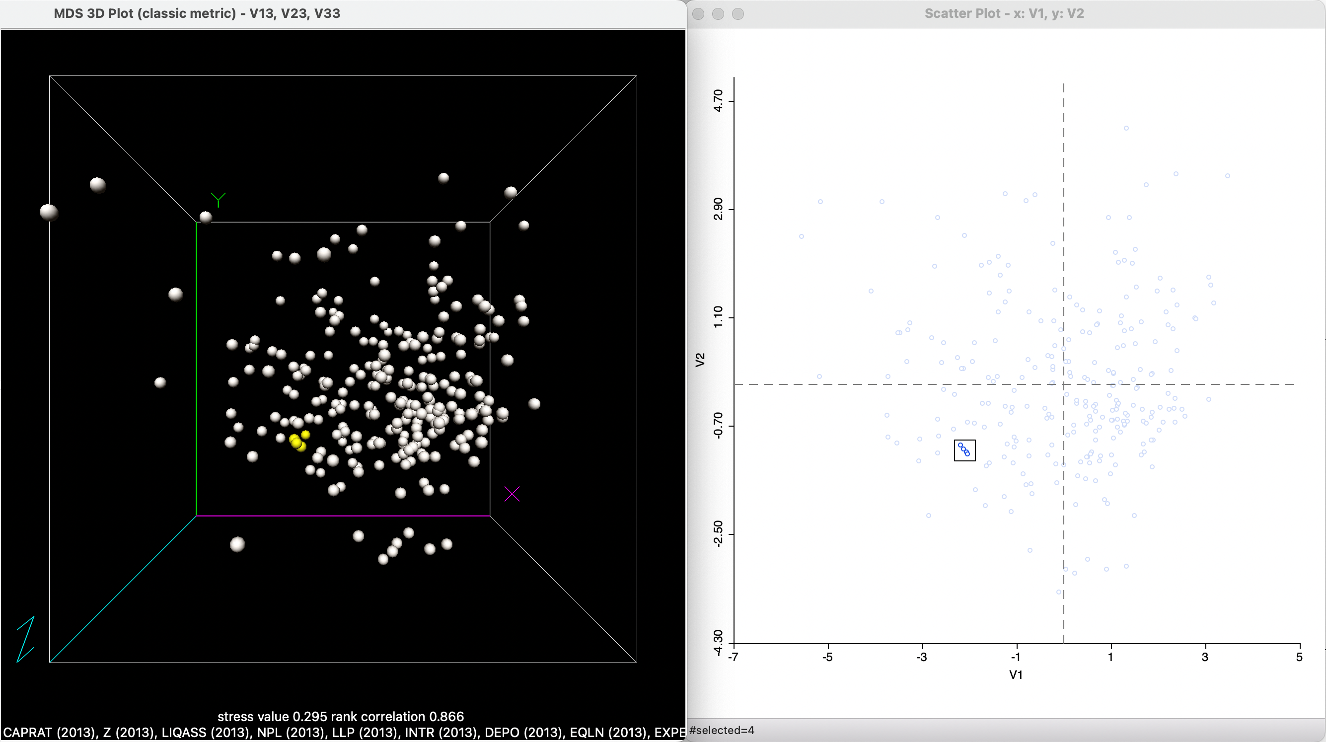
Figure 3.13: 3D MDS

For example, the rotation depicted in Figure 3.14 illustrates how a change in perspective can reveal larger distances in three dimensions that do not appear in the two-dimensional solution.

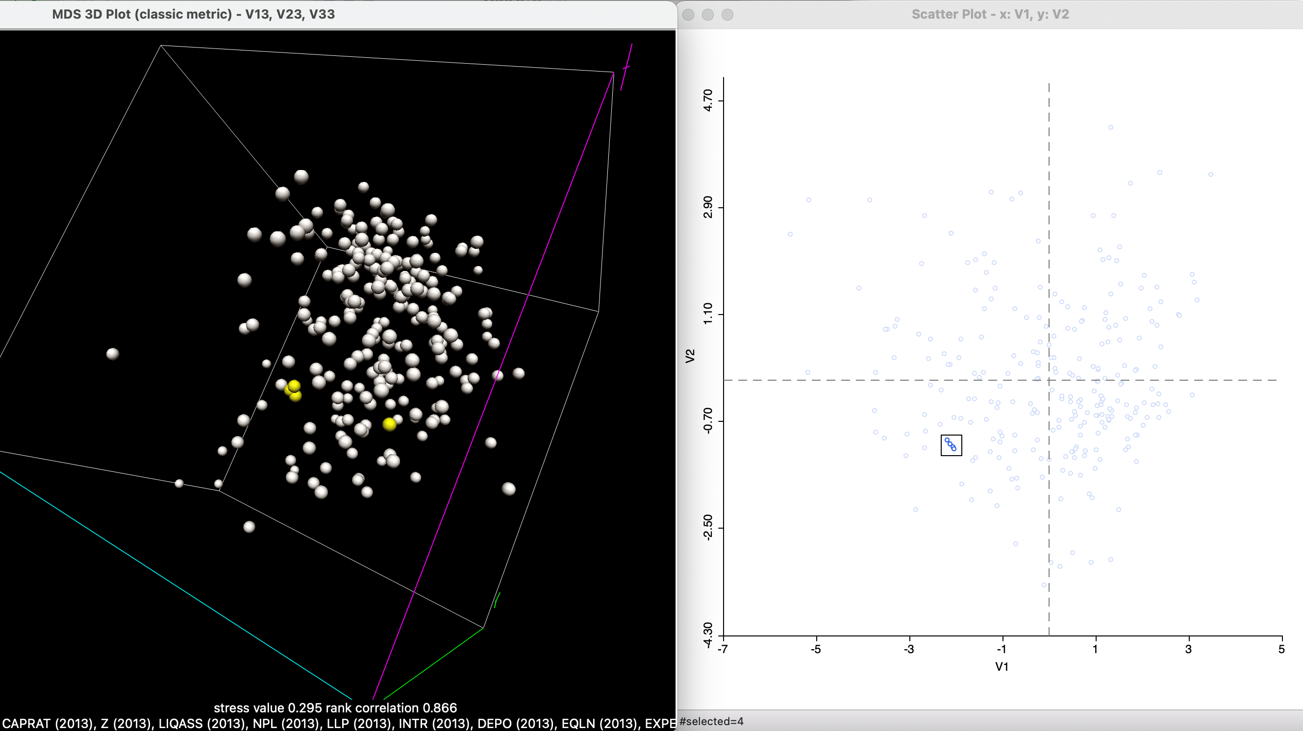
Figure 3.14: 3D MDS after Rotation