2.2 Matrix Algebra Review
Before moving on to the mathematics of principal components analysis, a brief review of some basic matrix algebra concepts is included here. Readers already familiar with this material can easily skip this section.
Vectors and matrices are ways to collect a lot of information and manipulate it in a concise mathematical way. One can think of a matrix as a table with rows and columns, and a vector as a single row or column. In two dimensions, i.e., for two values, a vector can be visualized as an arrow between the origin of the coordinate system (0,0) and a given point. The first value corresponds to the x-axis and the second value to the y-axis. In Figure 2.2, this is illustrated for the vector: \[ v = \begin{bmatrix} 1\\ 2 \end{bmatrix}. \] The arrow in the figure connects the origin of a \(x-y\) scatter plot to the point (\(x = 1\), \(y = 2\)).
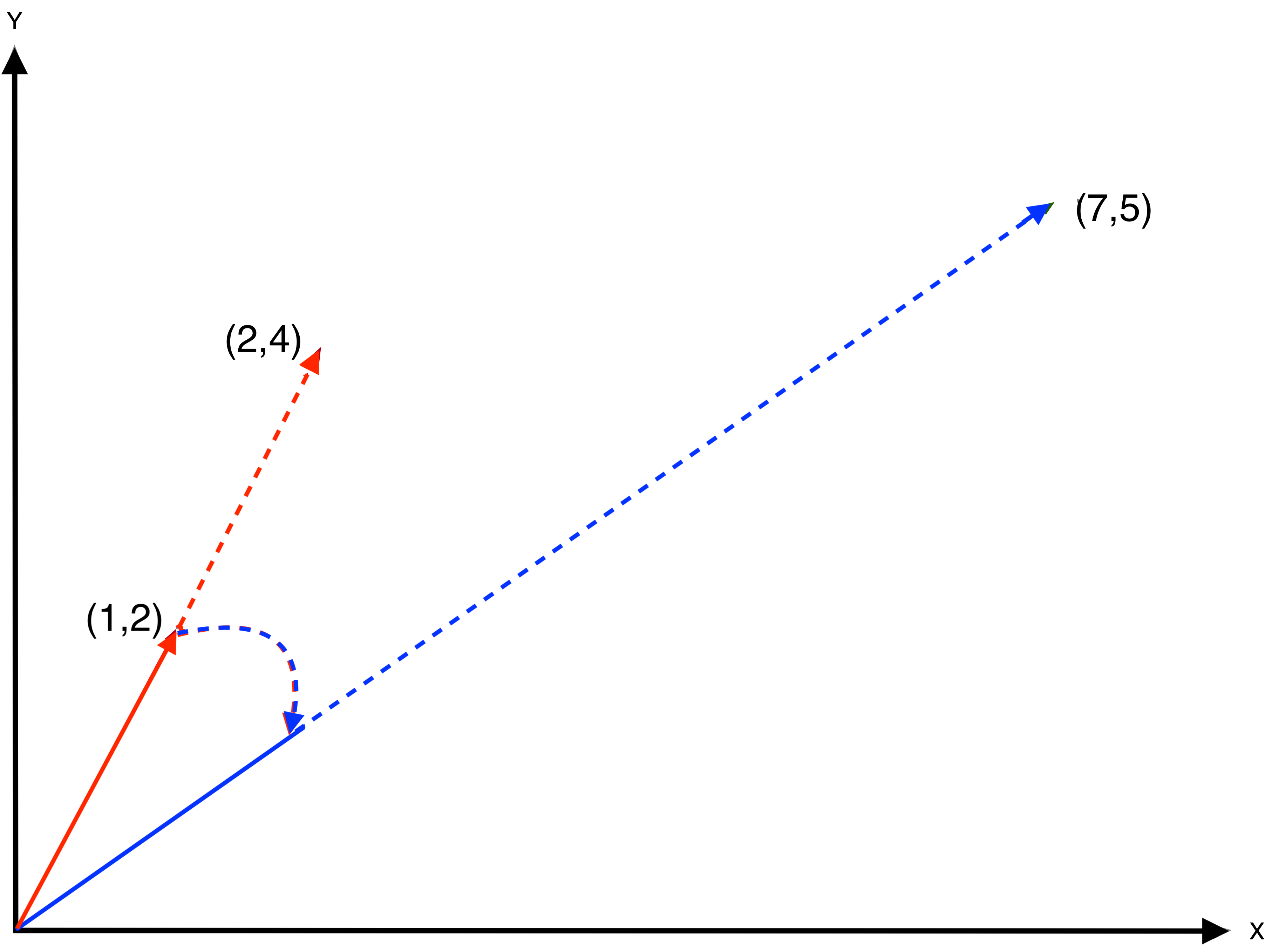
Figure 2.2: Vectors in Two-Dimensional Space
A central application in matrix algebra is the multiplication of vectors and matrices. The simplest case is the multiplication of a vector by a scalar (i.e., a single number). Graphically, multiplying a vector by a scalar just moves the end point further or closer on the same slope. For example, multiplying the vector \(v\) by the scalar \(2\) gives: \[ 2 \times \begin{bmatrix} 1\\ 2 \end{bmatrix} = \begin{bmatrix} 2\\ 4 \end{bmatrix} \] This is equivalent to moving the arrow over on the same slope from (1,2) to the point (2,4) further from the origin, as shown by the dashed red line in Figure 2.2.
Multiplying a matrix by a vector is slightly more complex, but again corresponds to a simple geometric transformation. For example, consider the \(2 \times 2\) matrix \(A\): \[ A = \begin{bmatrix} 1 & 3\\ 3 & 2 \end{bmatrix}. \] The result of a multiplication of a \(2 \times 2\) matrix by a \(2 \times 1\) column vector is a \(2 \times 1\) column vector. The first element of this vector is obtained as the product of the matching elements of the first row with the vector, the second element similarly as the product of the matching elements of the second row with the vector. In the example, this boils down to: \[ Av = \begin{bmatrix} (1 \times 1) + (3 \times 2)\\ (3 \times 1) + (2 \times 2) \end{bmatrix} = \begin{bmatrix} 7 \\ 5 \end{bmatrix}. \] Geometrically, this consists of a combination of rescaling and rotation. For example, in Figure 2.2, first the slope of the vector is changed, followed by a rescaling to the point (7,5), as shown by the blue dashed arrows.
A case of particular interest is for any matrix \(A\) to find a vector \(v\), such that when post-multiplied by that vector, there is only rescaling and no rotation. In other words, instead of finding what happens to the point (1,2) after pre-multiplying by the matrix \(A\), the interest focuses on finding a particular vector that just moves a point up or down on the same slope for that particular matrix. As it turns out, there are several such solutions. This problem is known as finding eigenvectors and eigenvalues for a matrix. It has a broad range of applications, including in the computation of principal components.
2.2.1 Eigenvalues and eigenvectors
The eigenvectors and eigenvalues of a square symmetric matrix \(A\) are a special scalar-vector pair, such that \(Av = \lambda v\), where \(\lambda\) is the eigenvalue and \(v\) is the eigenvector. In addition, the different eigenvectors are such that they are orthogonal to each other. This means that the product of two different eigenvectors is zero, i.e., \(v_u'v_k = 0\) (for \(u \neq k\)).1 Also, the sum of squares of the eigenvector elements equals one. In vector notation, \(v_u'v_u = 1\).
What does this mean? For an eigenvector (i.e., arrow from the origin), the transformation by \(A\) does not rotate the vector, but simply rescales it (i.e., moves it further or closer to the origin), by exactly the factor \(\lambda\).
For the example matrix \(A\), the two eigenvectors turn out to be [0.6464 0.7630] and [-0.7630 0.6464], with associated eigenvalues 4.541 and -1.541. Each square matrix has as many eigenvectors and matching eigenvalues as its rank, in this case 2 – for a 2 by 2 non-singular matrix. The actual computation of eigenvalues and eigenvectors is rather complicated, and is beyond the scope of this discussion.
To further illustrate this concept, consider post-multiplying the matrix \(A\) with its eigenvector [0.6464 0.7630]: \[ \begin{bmatrix} (1 \times 0.6464) + (3 \times 0.7630)\\ (3 \times 0.6464) + (2 \times 0.7630) \end{bmatrix} = \begin{bmatrix} 2.935\\ 3.465 \end{bmatrix} \] The eigenvector rescaled by the matching eigenvalue gives the same result: \[ 4.541 \times \begin{bmatrix} 0.6464\\ 0.7630 \end{bmatrix} = \begin{bmatrix} 2.935\\ 3.465 \end{bmatrix} \] In other words, for the point (0.6464 0.7630), a pre-multiplication by the matrix \(A\) just moves it by a multiple of 4.541 to a new location on the same slope, without any rotation.
With the eigenvectors stacked in a matrix \(V\), it is easy to verify that they are orthogonal and the sum of squares of the coefficients sum to one, i.e., \(V'V = I\) (with \(I\) as the identity matrix): \[ \begin{bmatrix} 0.6464 & -0.7630\\ 0.7630 & 0.6464 \end{bmatrix}' \begin{bmatrix} 0.6464 & -0.7630\\ 0.7630 & 0.6464 \end{bmatrix} = \begin{bmatrix} 1 & 0\\ 0 & 1 \end{bmatrix} \] In addition, it is easily verified that \(VV' = I\) as well. This means that the transpose of \(V\) is also its inverse (per the definition of an inverse matrix, i.e., a matrix for which the product with the original matrix yields the identity matrix), or \(V^{-1} = V'\).
Eigenvectors and eigenvalues are central in many statistical analyses, but it is important to realize they are not as complicated as they may seem at first sight. On the other hand, computing them efficiently is complicated, and best left to specialized programs.
Finally, a couple of useful properties of eigenvalues are worth mentioning.
The sum of the eigenvalues equals the trace of the matrix. The trace is the sum of the diagonal elements. For the matrix \(A\) in the example, the trace is \(1 + 2 = 3\). The sum of the two eigenvalues is \(4.541 -1.541 = 3\).
In addition, the product of the eigenvalues equals the determinant of the matrix. For a \(2 \times 2\) matrix, the determinant is \(ab - cd\), or the product of the diagonal elements minus the product of the off-diagonal elements. In the example, that is \((1 \times 2) - (3 \times 3) = -7\). The product of the two eigenvalues is \(4.541 \times -1.541 = -7.0\).
2.2.2 Matrix decompositions
In many applications in statistics and data science, a lot is gained by representing the original matrix by a product of special matrices, typically related to the eigenvectors and eigenvalues. These are so-called matrix decompositions. Two cases are particularly relevant for principal component analysis, as well as many other applications: spectral decomposition and singular value decomposition.
2.2.2.1 Spectral decomposition
For each eigenvector \(v\) of a square symmetric matrix \(A\), it holds that \(Av = \lambda v\). This can be written compactly for all the eigenvectors and eigenvalues by organizing the individual eigenvectors as columns in a \(k \times k\) matrix \(V\), with \(k\) as the dimension of the matrix \(A\). Similarly, the matching eigenvalues can be organized as the diagonal elements of a \(k \times k\) diagonal matrix, say \(G\).
The basic eigenvalue expression can then be written as \[AV = VG.\] Note that \(V\) goes first in the matrix multiplication on the right hand side to ensure that each column of \(V\) is multiplied by the corresponding eigenvalue on the diagonal of \(G\) to yield \(\lambda v\). Taking advantage of the fact that the eigenvectors are orthogonal, namely that \(VV' = I\), gives that post-multiplying each side of the equation by \(V'\) yields \(AVV' = VGV'\), or \[A = VGV'.\] This is the so-called eigenvalue decomposition or spectral decomposition of the square symmetric matrix \(A\).
For any \(n \times k\) matrix of standardized observations \(X\) (i.e., \(n\) observations on \(k\) variables), the square matrix \(X'X\) corresponds to the correlation matrix. The spectral decomposition of this matrix yields: \[X'X = VGV',\] with \(V\) as a matrix with the eigenvectors as columns, and \(G\) as a diagonal matrix containing the eigenvalues. This property can be used to construct the principal components of the matrix \(X\).
2.2.2.2 Singular value decomposition (SVD)
The spectral matrix decomposition only applies to square matrices. A more general decomposition is the so-called singular value decomposition, which applies to any rectangular matrix, such as the \(n \times k\) matrix \(X\) with (standardized) observations directly, rather than its correlation matrix.
For a full-rank \(n \times k\) matrix \(X\) (there are many more general cases where SVD can be applied), the decomposition takes the following form: \[X = UDV',\] where \(U\) is a \(n \times k\) orthonormal matrix (i.e., \(U'U = I\)), \(D\) is a \(k \times k\) diagonal matrix, and \(V\) is a \(k \times k\) orthonormal matrix (i.e., \(V'V = I\)).
While SVD is very general, the full generality is not needed for the PCA case. It turns out that there is a direct connection between the eigenvalues and eigenvectors of the (square) correlation matrix \(X'X\) and the SVD of \(X\). Using the SVD decomposition above, and exploiting the orthonormal properties of the various matrices, the product \(X'X\) can be written as: \[X'X = (UDV')'(UDV') = VDU'UDV' = VD^2V',\] since \(U'U = I\).
It thus turns out that the columns of \(V\) from the SVD decomposition contain the eigenvectors of \(X'X\). In addition, the square of the diagonal elements of \(D\) in the SVD are the eigenvalues of the correlation matrix. Or, equivalently, the diagonal elements of the matrix \(D\) are the square roots of the eigenvalues of \(X'X\). This property can be exploited to derive the principal components of the matrix \(X\).
The product of a row vector with a column vector is a scalar. The symbol \('\) stands for the transpose of a vector, in this case, a column vector that is turned into a row vector.↩︎