8.5 Implementation

Spectral clustering is invoked from the Clusters toolbar, as the next to last item in the classic clustering subset, shown in Figure 6.1. Alternatively, from the menu, it is selected as Clusters > Spectral.

The variable settings panel has the same general layout as for K-Means. The coordinates for the points are selected from the Select Variables dialog as x and y. In the Parameters panel, one set pertains to the construction of the Affinity (or adjacency) matrix, the others are the usual parameters for the K-Means algorithm that is applied to the transformed eigenvectors.

The Affinity option provides three alternatives, K-NN, Mutual K-NN and Gaussian, with specific parameters for each. In the example, the number of clusters is set to 2 and all options are kept to the default setting. This includes K-NN with 3 neighbors for the affinity matrix, and all the default settings for K-Means. The value of 3 for knn corresponds to \(\log_{10}(300) = 2.48\), rounded up to the next integer.

The Run button generates the cluster characteristics in the Summary panel. In the usual manner, this also brings up a new window with the cluster map, and saves the cluster classification as an integer variable to the data table.

8.5.1 Cluster results

The cluster map for the chosen parameter settings is shown in Figure 8.3. It yields a perfect separation of the two spirals, although that is by no means the case for all parameter settings, as will be illustrated below.

The cluster characteristics in Figure 8.4 list the parameter settings first, followed by the values for the cluster centers (the mean) for the two (standardized) coordinates and the decomposition of the sum of squares. The ratio of between sum of squares to total sum of squares is a dismal 0.04. This is not surprising, since this criterion provides a measure of the degree of compactness for the cluster, which a non-convex cluster like the spirals example does not meet.

In this example, it is easy to visually assess the extent to which the nonlinearity is captured. However, in the typical high-dimensional application, this will be much more of a challenge, since the usual measures of compactness may not be informative. A careful inspection of the distribution of the different variables across the observations in each cluster is therefore in order.

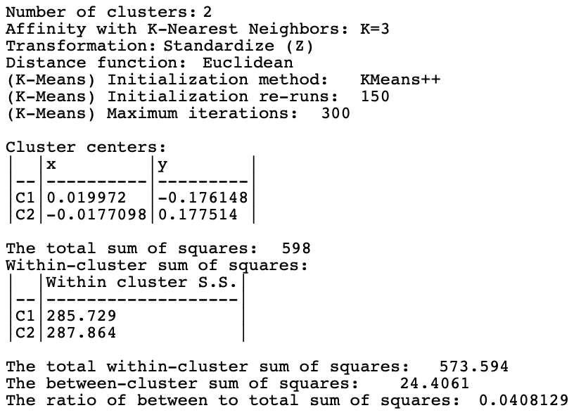
Figure 8.4: Cluster Characteristics for Spectral Clustering of Spirals Data - Default Settings

8.5.2 Options and Sensitivity Analysis

The results of spectral clustering are extremely sensitive to the parameters chosen to create the affinity matrix. Suggestions for default values are only suggestions, and the particular values many sometimes be totally unsuitable. Experimentation is therefor a necessity. There are two classes of parameters. One set pertains to the number of nearest Neighbors for K-NN or Mutual K-NN. The other set relates to the bandwidth of the Gaussian kernel, determined by the standard deviation Sigma.

8.5.2.1 K-nearest neighbor affinity matrix

The two default values for the number of nearest neighbors are contained in a drop-down list. In the spirals example, with n=300, \(\log_{10}(n) = 2.48\), which rounds up to 3, and \(\ln(n) = 5.70\), which rounds up to 6. These are the two default values provided. Any other value can be entered manually in the dialog. The options for a mutual knn affinity matrix have the same entries.

The results for the Mutual option with 3 nearest neighbors are shown in Figures 8.5 and 8.6. The separation is far from perfect, with cluster members in both spirals. The measures of fit are even worse than for the default case.

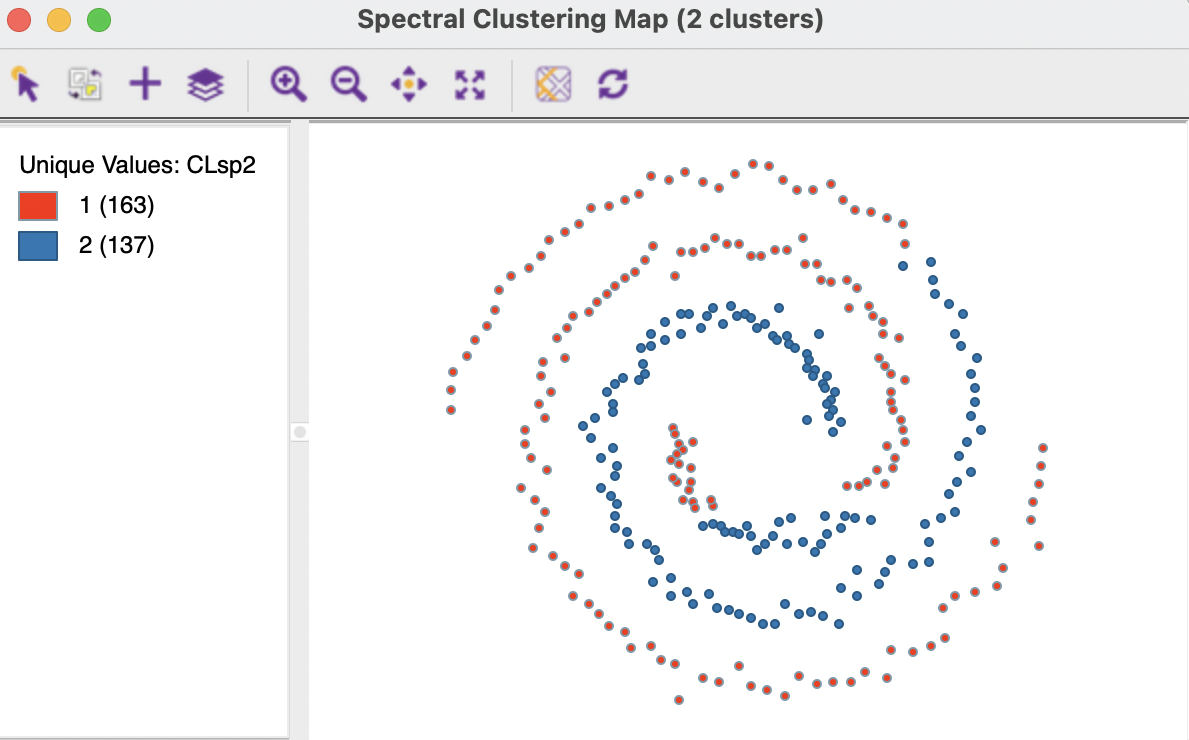
Figure 8.5: Cluster Characteristics for Spectral Clustering of Spirals Data - Mutual KNN=3

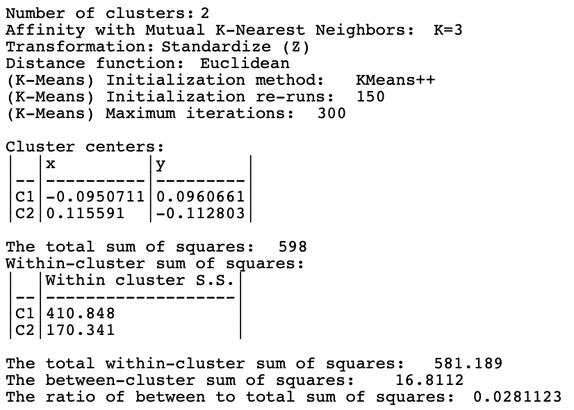
Figure 8.6: Cluster Characteristics for Spectral Clustering of Spirals Data - Mutual KNN=3

8.5.2.2 Gaussian kernel affinity matrix

The built-in options for sigma, the standard deviation of the Gaussian kernel are 0.707107, 3.477121, and 6.703782. The smallest value corresponds to \(\sqrt{1/p}\), where \(p\), the number of variables, equals 2 in the example. The other two values are \(\log_{10}(n) + 1\) and \(\ln(n) + 1\), yielding respectively 3.477121 and 6.703782 for n=300. In addition, any other value can be entered in the dialog.

The results for the first option (0.707107) are shown in Figures 8.7 and 8.8. The clusters totally fail to extract the shape of the separate spirals, although they are perfectly balanced. The layout looks similar to the results for K-Means and K-Medians in Figure 8.2. Interestingly, this layout scores much better on the BSS/TSS ratio (0.39). Rather than being an indication of a good separation, it suggests that the nonlinearity of the true clusters is not reflected in the grouping.

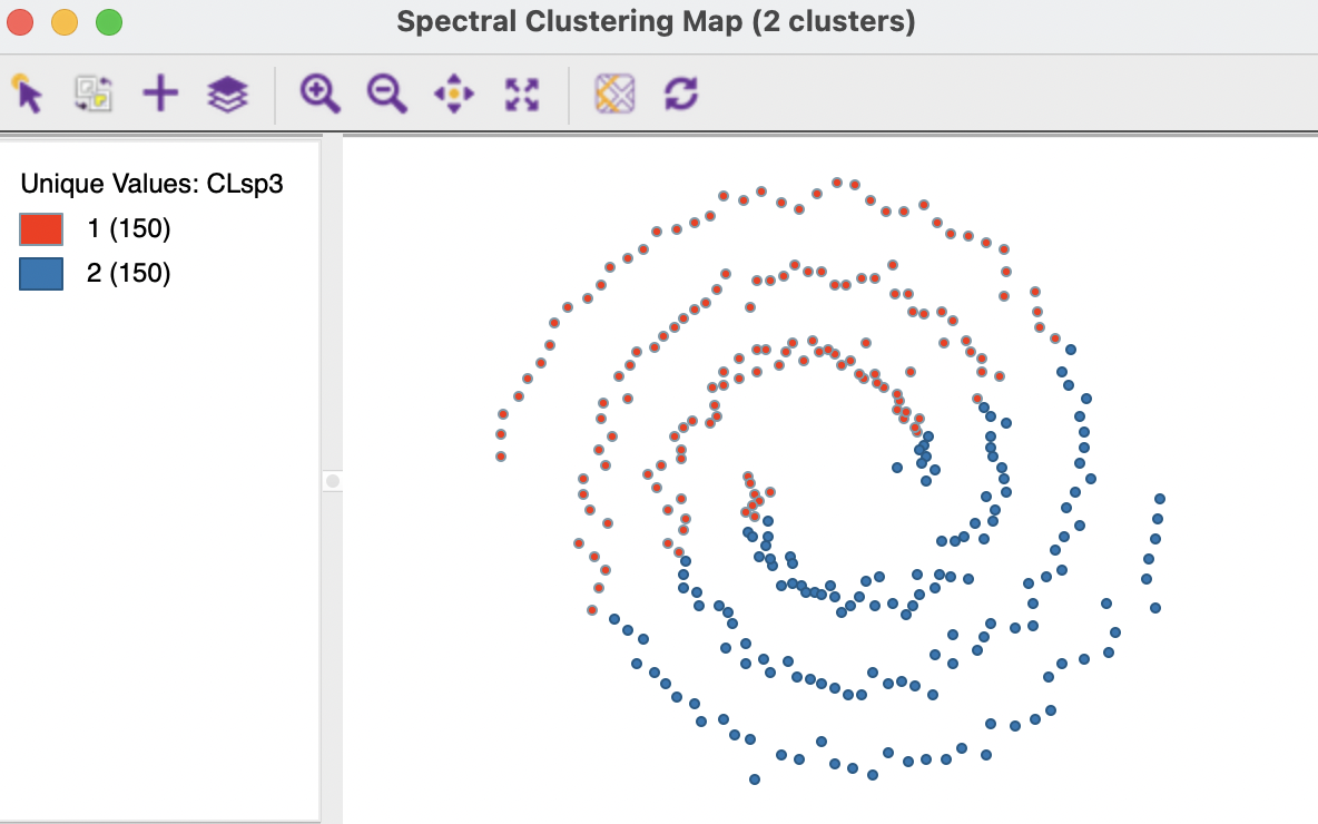
Figure 8.7: Cluster Characteristics for Spectral Clustering of Spirals Data - Gaussian Kernel

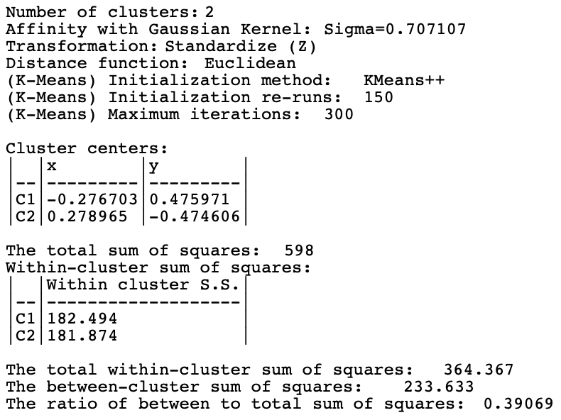
Figure 8.8: Cluster Characteristics for Spectral Clustering of Spirals Data - Gaussian Kernel

In order to find a solution that provides the same separation as in Figure 8.3, some experimentation with different values for \(\sigma\) is needed. As it turns out, the same result as for knn with 3 neighbors is obtained with \(\sigma = 0.08\) or \(0.07\), neither of which are even close to the default values. This illustrates how in an actual example, where the results cannot be readily visualized in two dimensions, it may be very difficult to find the parameter values that discover the true underlying patterns.